8 Quantum field theory

8.1 From Particles to Fields: Why Quantum Field Theory

Quantum mechanics nails atoms; special relativity nails fast things. Together, they disagree about headcount. Relativity allows particles to be created and destroyed; single-particle quantum mechanics does not. Quantum Field Theory (QFT) is the fix: the basic objects are fields, and particles are quanta (excitations) of those fields. This section sets the stage—why fields are necessary, how to quantize a simple field, how particles emerge, and which principles (locality, symmetry) keep everything sane.

8.1.1 What breaks if you stick with single-particle QM

Relativistic energy $E^{2}=p^{2}c^{2}+m^{2}c^{4}$ lets $E$ be negative, and a one-particle wave equation with a probability density you can trust is hard to maintain
Particle creation/annihilation. A high-energy photon turns into $e^{+}e^{-}$ ; an excited atom emits a photon. Fixed- $N$ Hilbert spaces cannot even describe these channels
Locality and causality. Measurements at spacelike separation should not influence each other. Enforcing this with only wavefunctions of a fixed number of particles gets messy fast

QFT resolves these by promoting fields to operators. States live in a Fock space where particle number can fluctuate, and microcausality is built into field commutators.

8.1.2 Fields as “infinitely many oscillators”

Take any free classical field, Fourier expand it into modes labeled by momentum $\boldsymbol k$ . Each mode is a harmonic oscillator. Quantization then is copy–paste from Chapter 7, but for every $\boldsymbol k$ . That is the whole vibe: quantize all the normal modes.

8.1.3 Classical warm-up: the Klein–Gordon field

For a real scalar field $\phi(x)$ with $x=(ct,\boldsymbol x)$ , the Lorentz-invariant action is

S[\phi] = \int d^{4}x\;\mathcal L,\qquad \mathcal L = \frac{1}{2}\,\partial_{\mu}\phi\,\partial^{\mu}\phi - \frac{1}{2}\,\frac{m^{2}c^{2}}{\hbar^{2}}\,\phi^{2}

Euler–Lagrange gives the Klein–Gordon (KG) equation

\left(\Box + \frac{m^{2}c^{2}}{\hbar^{2}}\right)\phi(x) = 0,\qquad \Box \equiv \partial_{\mu}\partial^{\mu}

Plane-wave solutions obey $k_{\mu}k^{\mu} = m^{2}c^{2}/\hbar^{2}$ , i.e., the relativistic dispersion.

8.1.4 Canonical quantization: equal-time brackets

Promote $\phi$ and its conjugate momentum

\pi(x) \equiv \frac{\partial \mathcal L}{\partial(\partial_{0}\phi)} = \partial_{0}\phi

to operators with equal-time commutation relations

[\hat\phi(t,\boldsymbol x),\hat\phi(t,\boldsymbol y)] = 0

[\hat\pi(t,\boldsymbol x),\hat\pi(t,\boldsymbol y)] = 0

[\hat\phi(t,\boldsymbol x),\hat\pi(t,\boldsymbol y)] = i\hbar\,\delta^{(3)}(\boldsymbol x-\boldsymbol y)

This is the field-theory clone of $[x,p]=i\hbar$ .

8.1.5 Mode expansion and creation/annihilation operators

Impose a large box of volume $V$ (later $V\to\infty$ ) and expand

\hat\phi(x) = \frac{1}{\sqrt{V}}\sum_{\boldsymbol k} \frac{1}{\sqrt{2\omega_{\boldsymbol k}}}\left(\hat a_{\boldsymbol k}\,e^{-i\omega_{\boldsymbol k} t + i\boldsymbol k\cdot\boldsymbol x} + \hat a_{\boldsymbol k}^{\dagger}\,e^{i\omega_{\boldsymbol k} t - i\boldsymbol k\cdot\boldsymbol x}\right)

with

\omega_{\boldsymbol k} = \sqrt{c^{2}\boldsymbol k^{2} + \frac{m^{2}c^{4}}{\hbar^{2}}}

Choose the normalization so that

[\hat a_{\boldsymbol k},\hat a_{\boldsymbol k'}^{\dagger}] = \delta_{\boldsymbol k\boldsymbol k'},\qquad [\hat a_{\boldsymbol k},\hat a_{\boldsymbol k'}] = 0,\qquad [\hat a_{\boldsymbol k}^{\dagger},\hat a_{\boldsymbol k'}^{\dagger}] = 0

Exactly the oscillator algebra from §7.3, now for every momentum.

8.1.6 Fock space and particles

Define the vacuum by $\hat a_{\boldsymbol k}\ket{0}=0$ . One-particle states are

\ket{\boldsymbol k} \equiv \hat a_{\boldsymbol k}^{\dagger}\ket{0}

and multi-particle states follow by applying more creation operators. The number operator for mode $\boldsymbol k$ is $\hat N_{\boldsymbol k}=\hat a_{\boldsymbol k}^{\dagger}\hat a_{\boldsymbol k}$ . The Hamiltonian of the free field is

\hat H = \sum_{\boldsymbol k}\hbar\omega_{\boldsymbol k}\left(\hat a_{\boldsymbol k}^{\dagger}\hat a_{\boldsymbol k} + \frac{1}{2}\right)

The $\tfrac12$ term stacks up over all modes: vacuum energy. We will normally normal order to drop it in non-gravitational problems.

8.1.7 Normal ordering and vacuum energy

Define normal ordering $:\cdots:$ by placing all $\hat a^{\dagger}$ to the left of all $\hat a$ . Then

:\hat a_{\boldsymbol k}^{\dagger}\hat a_{\boldsymbol k}: = \hat a_{\boldsymbol k}^{\dagger}\hat a_{\boldsymbol k}

and

:\hat H: = \sum_{\boldsymbol k}\hbar\omega_{\boldsymbol k}\,\hat a_{\boldsymbol k}^{\dagger}\hat a_{\boldsymbol k}

This sets the vacuum energy to zero by convention. In curved spacetime or gravity you must confront the absolute value; in flat-space particle physics we care about differences, so normal ordering is fine.

8.1.8 Locality and microcausality

A core QFT requirement is microcausality:

[\hat\phi(x),\hat\phi(y)] = 0\quad\text{for}\quad (x-y)^{2}<0

i.e., fields commute at spacelike separation. For the free KG field, the commutator is a c-number that vanishes outside the light cone. This is how QFT bakes in “no faster-than-light influence” at the operator level.

8.1.9 Green’s functions and propagators

Correlation functions encode everything. The time-ordered two-point function (Feynman propagator) is

i\Delta_{F}(x-y) \equiv \langle 0|\,T\{\hat\phi(x)\hat\phi(y)\}\,|0\rangle

It is the Green’s function of the KG operator:

\left(\Box + \frac{m^{2}c^{2}}{\hbar^{2}}\right)\Delta_{F}(x-y) = -\,\delta^{(4)}(x-y)

In momentum space,

\Delta_{F}(k) = \frac{i}{k^{2} - \frac{m^{2}c^{2}}{\hbar^{2}} + i\epsilon}

Poles at the mass shell and the $i\epsilon$ tell you how to go around them—causality in complex analysis clothing.

8.1.10 Noether currents and the stress tensor

Continuous symmetries of the action yield conserved currents. For spacetime translations we get the energy–momentum tensor $T^{\mu\nu}$ . One convenient symmetric form is

T^{\mu\nu} = \partial^{\mu}\phi\,\partial^{\nu}\phi - \eta^{\mu\nu}\,\mathcal L

satisfying $\partial_{\mu}T^{\mu\nu}=0$ . The conserved charges are 4-momentum

P^{\nu} = \int d^{3}x\;T^{0\nu}

which acts as the generator of spacetime translations on fields.

If $\phi$ is complex with a global $U(1)$ symmetry $\phi\to e^{i\alpha}\phi$ , you also get a conserved Noether current and charge (particle number for free fields).

8.1.11 Bosons, fermions, and the spin–statistics rule

Empirically and theoretically: integer-spin fields quantize with commutators (bosons), half-integer-spin fields with anticommutators (fermions). For a spinor $\psi$ , equal-time brackets are

\{\hat\psi_{\alpha}(t,\boldsymbol x),\hat\psi_{\beta}^{\dagger}(t,\boldsymbol y)\} = \delta_{\alpha\beta}\,\delta^{(3)}(\boldsymbol x-\boldsymbol y)

This choice is not optional decoration—spin–statistics plus locality and positivity force it.

8.1.12 How interactions enter (preview)

Add interaction terms to the Lagrangian, e.g., for a scalar

\mathcal L = \frac{1}{2}\,\partial_{\mu}\phi\,\partial^{\mu}\phi - \frac{1}{2}\,m^{2}\phi^{2} - \frac{\lambda}{4!}\,\phi^{4}

or couple fields, e.g., Yukawa $\bar\psi\psi\phi$ or gauge couplings via covariant derivatives. Perturbation theory then expands correlation functions into Feynman diagrams, with propagators as lines and couplings as vertices. Renormalization cleans divergences and defines physical parameters.

8.1.13 Worked mini-examples

(a) One-particle normalization.
Show $\langle \boldsymbol k'|\boldsymbol k\rangle = \delta_{\boldsymbol k'\boldsymbol k}$ using the $[\hat a,\hat a^{\dagger}]$ algebra.

(b) Vacuum two-point function.
Insert the mode expansion into $\langle 0|T\{\hat\phi(x)\hat\phi(y)\}|0\rangle$ to derive $\Delta_{F}(x-y)$ and its momentum-space form.

(c) Microcausality check.
Compute $[\hat\phi(x),\hat\phi(y)]$ for the free field; show it vanishes when $(x-y)^{2}<0$ by contour integration.

(d) Energy of a one-quantum state.
Act with $\hat H$ on $\ket{\boldsymbol k}$ and confirm $E=\hbar\omega_{\boldsymbol k}$ .

8.1.14 Minimal problem kit

Starting from $\mathcal L=\tfrac12(\partial\phi)^{2}-\tfrac12 m^{2}\phi^{2}$ , derive the canonical momentum $\pi$ and equal-time commutators that reproduce the mode algebra
Quantize a complex scalar field; identify the conserved $U(1)$ charge operator and show it counts particles minus antiparticles
Compute the retarded Green’s function $\Delta_{R}(x)$ and compare its support with $\Delta_{F}(x)$
Show that normal ordering removes the vacuum energy from $\hat H$ but not from $T^{\mu\nu}$ ’s trace unless you add counterterms
For a scalar with periodic boundary conditions in a box, replace the sum by an integral as $V\to\infty$ and recover continuum delta functions

8.2 The Dirac Field: Spinors, Anticommutators, and Relativistic Fermions

To describe electrons (and every spin- $\tfrac12$ particle) in a way that respects quantum mechanics and special relativity, we need fields with spinor degrees of freedom and anticommutation at equal time. Dirac’s equation supplies both, predicts antiparticles, and bakes $g\approx 2$ for the magnetic moment right into the cake. In this section we set up the algebra, solutions, quantization, currents, and the nonrelativistic limit.

Unit choice: we will use natural units $\hbar=c=1$ for compactness unless otherwise stated. You can restore $\hbar$ and $c$ by dimensional analysis.

8.2.1 Motivation in one page

Klein–Gordon waves handle relativity but describe spin-0 and permit negative densities. We want a first-order equation in time with a positive-definite probability density, consistent with $E^{2}=\boldsymbol p^{2}+m^{2}$ . Dirac’s idea: linearize the relativistic dispersion with matrices obeying a new algebra.

8.2.2 Gamma matrices and the Clifford algebra

Introduce $4\times4$ matrices $\gamma^{\mu}$ obeying

\{\gamma^{\mu},\gamma^{\nu}\} \equiv \gamma^{\mu}\gamma^{\nu}+\gamma^{\nu}\gamma^{\mu} = 2\,\eta^{\mu\nu}\,\mathbb I

with metric $\eta^{\mu\nu}=\mathrm{diag}(+,-,-,-)$ . Two common representations:

Dirac basis: $\gamma^{0}=\begin{pmatrix}\mathbb I&0\\0&-\mathbb I\end{pmatrix}$ , $\gamma^{i}=\begin{pmatrix}0&\sigma^{i}\\-\,\sigma^{i}&0\end{pmatrix}$
Chiral (Weyl) basis: $\gamma^{0}=\begin{pmatrix}0&\mathbb I\\ \mathbb I&0\end{pmatrix}$ , $\gamma^{i}=\begin{pmatrix}0&\sigma^{i}\\ -\sigma^{i}&0\end{pmatrix}$

Define

\gamma^{5} \equiv i\gamma^{0}\gamma^{1}\gamma^{2}\gamma^{3},\qquad (\gamma^{5})^{2}=1,\qquad \{\gamma^{5},\gamma^{\mu}\}=0

and the sigma matrices

\sigma^{\mu\nu} \equiv \frac{i}{2}\,[\gamma^{\mu},\gamma^{\nu}]

8.2.3 Dirac equation, adjoint, and Lagrangian

The Dirac equation for a spinor field $\psi(x)$ is

(i\gamma^{\mu}\partial_{\mu} - m)\,\psi(x) = 0

Define the adjoint $\bar\psi \equiv \psi^{\dagger}\gamma^{0}$ . The Lorentz-invariant Lagrangian is

\mathcal L = \bar\psi\,(i\gamma^{\mu}\partial_{\mu} - m)\,\psi

Varying $\bar\psi$ gives Dirac’s equation; varying $\psi$ gives the adjoint equation $\bar\psi\,(i\overleftarrow{\partial}_{\mu}\gamma^{\mu}+m)=0$ .

Conserved current by Noether’s theorem (global $U(1)$ phase):

j^{\mu} = \bar\psi\,\gamma^{\mu}\,\psi,\qquad \partial_{\mu}j^{\mu}=0

$j^{0}=\psi^{\dagger}\psi$ is positive-definite for solutions, delivering a proper probability density.

8.2.4 Plane-wave spinors and completeness

Seek plane waves $\psi=u_{s}(p)\,e^{-ip\cdot x}$ and $\psi=v_{s}(p)\,e^{+ip\cdot x}$ with on-shell $p^{2}=m^{2}$ . They satisfy

(/\!\!p - m)\,u_{s}(p) = 0,\qquad (/\!\!p + m)\,v_{s}(p) = 0

where $/\!\!p\equiv \gamma^{\mu}p_{\mu}$ and $s$ labels spin. Normalizations convenient for QFT:

\bar u_{s}(p)\,u_{s'}(p)=2m\,\delta_{ss'},\qquad \bar v_{s}(p)\,v_{s'}(p)=-2m\,\delta_{ss'}

Spin sums (completeness):

\sum_{s} u_{s}(p)\,\bar u_{s}(p) = /\!\!p + m

\sum_{s} v_{s}(p)\,\bar v_{s}(p) = /\!\!p - m

These identities are the workhorses behind cross sections and propagators.

8.2.5 Minimal coupling and the Pauli term (sneak peek)

Electromagnetism enters via the covariant derivative $D_{\mu}=\partial_{\mu}+ieA_{\mu}$ . The Dirac equation becomes $(i\gamma^{\mu}D_{\mu}-m)\psi=0$ and the Lagrangian $\mathcal L=\bar\psi(i\gamma^{\mu}D_{\mu}-m)\psi$ . In the nonrelativistic limit this yields a magnetic interaction with moment

\boldsymbol{\mu} = g\,\frac{e}{2m}\,\boldsymbol S,\qquad g_{\text{Dirac}}=2

Radiative corrections in QED make $g=2(1+a_{e})$ with tiny $a_{e}$ .

8.2.6 Canonical quantization and anticommutators

Promote $\psi$ to an operator field; impose equal-time anticommutation:

\{\hat\psi_{\alpha}(t,\boldsymbol x),\hat\psi_{\beta}^{\dagger}(t,\boldsymbol y)\} = \delta_{\alpha\beta}\,\delta^{(3)}(\boldsymbol x-\boldsymbol y)

\{\hat\psi,\hat\psi\}=\{\hat\psi^{\dagger},\hat\psi^{\dagger}\}=0

Expand in modes (box normalization; later $\sum\to\int$ ):

\hat\psi(x) = \sum_{s}\int\!\frac{d^{3}\boldsymbol p}{(2\pi)^{3}}\;\frac{1}{\sqrt{2E_{\boldsymbol p}}}\left[ \hat b_{s}(\boldsymbol p)\,u_{s}(p)\,e^{-ip\cdot x} + \hat d_{s}^{\dagger}(\boldsymbol p)\,v_{s}(p)\,e^{+ip\cdot x}\right]

with $E_{\boldsymbol p}=\sqrt{\boldsymbol p^{2}+m^{2}}$ and

\{\hat b_{s}(\boldsymbol p),\hat b_{s'}^{\dagger}(\boldsymbol p')\}=(2\pi)^{3}\delta_{ss'}\delta^{(3)}(\boldsymbol p-\boldsymbol p')

\{\hat d_{s}(\boldsymbol p),\hat d_{s'}^{\dagger}(\boldsymbol p')\}=(2\pi)^{3}\delta_{ss'}\delta^{(3)}(\boldsymbol p-\boldsymbol p')

All other anticommutators vanish. Here $\hat b^{\dagger}$ creates a particle and $\hat d^{\dagger}$ an antiparticle.

The normal-ordered Hamiltonian reads

:\hat H: = \sum_{s}\int\!\frac{d^{3}\boldsymbol p}{(2\pi)^{3}}\;E_{\boldsymbol p}\left[\hat b_{s}^{\dagger}(\boldsymbol p)\hat b_{s}(\boldsymbol p)+\hat d_{s}^{\dagger}(\boldsymbol p)\hat d_{s}(\boldsymbol p)\right]

8.2.7 Propagator and Feynman rules

The time-ordered two-point function (Dirac propagator) is

S_{F}(x-y) \equiv \langle 0|\,T\{\hat\psi(x)\,\bar{\hat\psi}(y)\}\,|0\rangle

In momentum space,

S_{F}(p) = \frac{i}{/\!\!p - m + i\epsilon} = i\,\frac{/\!\!p+m}{p^{2}-m^{2}+i\epsilon}

A free Dirac line in a Feynman diagram carries this factor; interactions insert vertices (e.g., $-ie\gamma^{\mu}$ for QED).

A free Dirac line in a Feynman diagram

8.2.8 Bilinears, currents, and Gordon identity

Useful bilinears and their transformation properties:

Scalar $\bar\psi\psi$
Pseudoscalar $i\bar\psi\gamma^{5}\psi$
Vector $\bar\psi\gamma^{\mu}\psi$
Axial vector $\bar\psi\gamma^{\mu}\gamma^{5}\psi$
Tensor $\bar\psi\sigma^{\mu\nu}\psi$

Vector current is conserved for global phase symmetry. The Gordon identity relates vector currents to orbital plus spin pieces:

\bar u(p')\,\gamma^{\mu}\,u(p) = \frac{1}{2m}\,\bar u(p')\!\left[(p'+p)^{\mu} + i\,\sigma^{\mu\nu}(p'-p)_{\nu}\right]\!u(p)

It is the algebraic source of the Pauli magnetic term in low-energy expansions.

8.2.9 Chirality, helicity, and the massless limit

Define chiral projectors

P_{L}=\frac{1-\gamma^{5}}{2},\qquad P_{R}=\frac{1+\gamma^{5}}{2}

Left/right components $\psi_{L,R}=P_{L,R}\psi$ decouple when $m=0$ . Helicity (spin along momentum) equals chirality only for massless states. The Standard Model’s weak interactions couple to $\psi_{L}$ but not $\psi_{R}$ for leptons—chirality matters.

Majorana vs Dirac. A Majorana field satisfies $\psi^{c}=\psi$ (equal to its charge conjugate) and has no independent antiparticle. Dirac fields (like the electron) carry a conserved $U(1)$ charge.

8.2.10 Discrete symmetries $C$ , $P$ , and $T$ (sketch)

Implementations depend on representation up to phases:

Parity $P$ : $\psi(t,\mathbf x)\to \gamma^{0}\psi(t,-\mathbf x)$
Charge conjugation $C$ : $\psi \to C\,\bar\psi^{T}$ with $C^{-1}\gamma^{\mu}C=-(\gamma^{\mu})^{T}$
Time reversal $T$ : antiunitary; roughly $\psi(t,\mathbf x)\to i\gamma^{1}\gamma^{3}\psi^{\ast}(-t,\mathbf x)$ in Dirac basis

Local Lorentz-invariant interactions built from the bilinears can be classified by their $C$ , $P$ , $T$ parities.

8.2.11 Nonrelativistic limit → Pauli equation

Insert minimal coupling $D_{\mu}$ and separate “large” and “small” components in the Dirac basis. Eliminating the small component to order $1/m$ yields the Pauli Hamiltonian

H_{\text{Pauli}} = \frac{1}{2m}\,(\boldsymbol p - e\boldsymbol A)^{2} + e\phi - \frac{e}{2m}\,\boldsymbol{\sigma}\cdot \boldsymbol B

with $\boldsymbol B=\nabla\times\boldsymbol A$ . The $\boldsymbol{\sigma}\cdot\boldsymbol B$ term gives $g=2$ at tree level. Higher orders add spin–orbit and Darwin terms (matching hydrogen fine structure).

8.2.12 Worked mini-examples

(a) Current conservation.
Use Dirac’s equation and its adjoint to show $\partial_{\mu}(\bar\psi\gamma^{\mu}\psi)=0$ .

(b) Propagator inversion.
Check that $(/\!\!p-m)\,[(/\!\!p+m)/(p^{2}-m^{2})] = \mathbb I$ .

(c) Spin sums.
Prove $\sum_{s}u_{s}(p)\bar u_{s}(p)=/\!\!p+m$ by completeness of plane-wave solutions.

(d) Pauli reduction.
Starting from $(\boldsymbol{\alpha}\cdot\boldsymbol{\pi}+ \beta m + e\phi)\psi=i\partial_{t}\psi$ , with $\boldsymbol{\pi}=\boldsymbol p-e\boldsymbol A$ , eliminate the small component to order $1/m$ and recover $-\tfrac{e}{2m}\boldsymbol{\sigma}\cdot\boldsymbol B$ .

(e) Helicity conservation for $m=0$ .
Show that $[H,\boldsymbol{\Sigma}\cdot \hat{\boldsymbol p}]=0$ for the free massless Dirac Hamiltonian, so helicity is conserved.

8.2.13 Minimal problem kit

Verify the Clifford algebra for the explicit Dirac or chiral gamma matrices and compute $\gamma^{5}$
Derive the mode expansion coefficients by projecting $\hat\psi$ onto $u_{s}(p)$ and $v_{s}(p)$ ; recover the $\{\hat b,\hat b^{\dagger}\}$ and $\{\hat d,\hat d^{\dagger}\}$ algebras
Using the Gordon identity, extract the nonrelativistic limit of the electromagnetic current and identify the spin magnetic moment term
Classify the bilinears $\bar\psi\Gamma\psi$ by $C$ , $P$ , and $T$ transformation properties
Show explicitly that the mass term $m\bar\psi\psi$ mixes chiralities while $\bar\psi\gamma^{\mu}\psi$ does not
For a Majorana field, write the reality condition in the chiral basis and count on-shell degrees of freedom versus a Dirac field

8.2A Weyl and Majorana Spinors: Two-Component Life, Mass Terms, and DOF Counting

Dirac spinors are great, but a lot of real work is tidier in two-component language. In the chiral basis a Dirac spinor splits as $\psi = \begin{pmatrix}\chi\\ \phi\end{pmatrix}$ with left/right Weyl spinors $\chi$ and $\phi$ .

8.2A.1 Weyl equations and helicity

For a massless fermion, left and right components decouple:

i\,\sigma^{\mu}\partial_{\mu}\,\chi = 0,\qquad i\,\bar\sigma^{\mu}\partial_{\mu}\,\phi = 0

with $\sigma^{\mu}=(\mathbb I,\boldsymbol{\sigma})$ and $\bar\sigma^{\mu}=(\mathbb I,-\boldsymbol{\sigma})$ . A single Weyl field has two on-shell degrees of freedom: particle and antiparticle with fixed chirality; for $m=0$ helicity equals chirality.

8.2A.2 Dirac mass and how it mixes chiralities

The Dirac mass term in two-component form reads

\mathcal L_{m_D} = -\,m_D\left(\chi^{\dagger}\phi + \phi^{\dagger}\chi\right)

It preserves a global $U(1)$ (fermion number) and couples $\chi$ to $\phi$ . Turning it on fuses the two Weyl fields into one Dirac fermion.

8.2A.3 Majorana mass and reality condition

Charge conjugation acts as $\psi^{c} \equiv C\,\bar\psi^{T}$ . A Majorana fermion satisfies the reality condition

\psi = \psi^{c}

In two-component form one can write a Majorana mass for a single Weyl field, e.g. for left chirality

\mathcal L_{m_M} = -\,\frac{1}{2}\,m_M\left(\chi^{T} i\sigma^{2}\chi + \chi^{\dagger} i\sigma^{2}\chi^{\ast}\right)

It violates the $U(1)$ number symmetry (particle $\leftrightarrow$ antiparticle are the same). You can also combine Dirac and Majorana masses to get seesaw patterns.

8.2A.4 Degrees of freedom: the headcount

Dirac: 4 on-shell states = 2 spin $\times$ (particle, antiparticle)
Majorana: 2 on-shell states = 2 spin, but particle is its own antiparticle
Massless Weyl: 2 on-shell states tied to one chirality; helicity fixed in the massless limit

8.2A.5 Handy identities in two components

Spinor contractions use $\epsilon^{ab}$ ( $\epsilon^{12}=+1$ ). Some workhorse relations:

\sigma^{\mu}\bar\sigma^{\nu} + \sigma^{\nu}\bar\sigma^{\mu} = 2\eta^{\mu\nu}\,\mathbb I,\qquad \bar\sigma^{\mu}\sigma^{\nu} + \bar\sigma^{\nu}\sigma^{\mu} = 2\eta^{\mu\nu}\,\mathbb I

For momenta $p\cdot\sigma \equiv p_{\mu}\sigma^{\mu}$ and $p\cdot\bar\sigma \equiv p_{\mu}\bar\sigma^{\mu}$ ,

(p\cdot\sigma)(p\cdot\bar\sigma) = p^{2}\,\mathbb I

These let you shuttle between 2-spinor and 4-spinor algebra without tears.

8.2A.6 Problem kit

Show that a Majorana mass is incompatible with a conserved global $U(1)$ for the same field
Derive the Dirac mass term $\bar\psi\psi$ from the two-component expression above
Prove that for $m=0$ the helicity operator equals chirality on plane-wave solutions
Count physical DOF for Dirac vs Majorana by explicitly building one-particle states

In summary: Weyl spinors are the minimal chiral building blocks; Dirac mass glues left and right; Majorana mass glues a field to its own charge conjugate and kills $U(1)$ number. The bookkeeping becomes simple, and many symmetry arguments are clearer in two components.

8.2B Discrete Symmetries Cheat Sheet: $C$ , $P$ , $T$ on Spinors and Bilinears

Discrete symmetries organize what interactions are allowed. Here’s a compact map. Conventions below match a common choice (Dirac basis phases); $T$ is antiunitary—overall signs can depend on phase conventions, but the pattern is standard.

8.2B.1 Actions on fields (one standard convention)

Parity $P$ : $\psi(t,\mathbf x)\to \gamma^{0}\psi(t,-\mathbf x)$ , $\bar\psi\to \bar\psi(t,-\mathbf x)\gamma^{0}$
Charge conjugation $C$ : $\psi \to C\,\bar\psi^{T}$ , $\bar\psi \to -\,\psi^{T} C^{-1}$ , with $C^{-1}\gamma^{\mu}C = -(\gamma^{\mu})^{T}$
Time reversal $T$ : $\psi(t,\mathbf x)\to i\gamma^{1}\gamma^{3}\,\psi^{\ast}(-t,\mathbf x)$ (antiunitary)

8.2B.2 Bilinear dictionary and transformation signs

Define bilinears

Scalar $S=\bar\psi\psi$
Pseudoscalar $P=i\bar\psi\gamma^{5}\psi$
Vector $V^{\mu}=\bar\psi\gamma^{\mu}\psi$
Axial $A^{\mu}=\bar\psi\gamma^{\mu}\gamma^{5}\psi$
Tensor $T^{\mu\nu}=\bar\psi\sigma^{\mu\nu}\psi$ , with $\sigma^{\mu\nu}=\tfrac{i}{2}[\gamma^{\mu},\gamma^{\nu}]$

Under $C$ (charge conjugation):

$S$ : even
$P$ : even
$V^{\mu}$ : odd
$A^{\mu}$ : even
$T^{\mu\nu}$ : odd

Under $P$ (parity):

$S$ : even
$P$ : odd
$V^{0}$ : even, $V^{i}$ : odd
$A^{0}$ : odd, $A^{i}$ : even
$T^{0i}$ : odd, $T^{ij}$ : even

Under $T$ (time reversal; antiunitary, standard convention):

$S$ : even
$P$ : odd
$V^{0}$ : even, $V^{i}$ : odd
$A^{0}$ : odd, $A^{i}$ : even
$T^{0i}$ : even, $T^{ij}$ : odd

Sanity checks: $CP$ sends $P$ (pseudoscalar) to odd, as used in axion and $\theta$ -term lore; $CPT$ keeps any Lorentz-invariant local Lagrangian density invariant.

8.2B.3 Quick uses

Building model terms: to be $CP$ -even with fermions, stick to $S$ , $V^{\mu}$ with appropriate contractions; $P$ and $A^{\mu}$ introduce $CP$ -odd structures
Spectroscopy: classify transitions by $J^{PC}$ using bilinears as interpolating operators
EDM tests: an electron electric dipole moment operator $\bar\psi i\sigma^{\mu\nu}\gamma^{5}\psi\,F_{\mu\nu}$ is $P$ - and $T$ -odd → a clean $CP$ -violation probe via $CPT$

8.2B.4 Problem kit

Derive the $C$ -parity of $V^{\mu}$ using $C^{-1}\gamma^{\mu}C=-(\gamma^{\mu})^{T}$
Show the $P$ -sign flip between $V^{0}$ and $V^{i}$ from explicit spatial inversion
Using antiunitarity of $T$ (complex conjugation), track the extra sign on the pseudoscalar
Classify the $C$ , $P$ , $T$ properties of $\bar\psi\sigma^{\mu\nu}\gamma^{5}\psi$ and relate it to dual tensors $\tilde F^{\mu\nu}$

In summary: With a fixed convention, $C$ , $P$ , and $T$ act predictably on the five basic bilinears. This table is your instant filter for which operators respect or violate given discrete symmetries.

8.2C QED Vertex and the Ward Identity: Gauge Invariance in One Page

Minimal coupling makes electromagnetism almost embarrassingly simple in QFT—and the Ward identity is the algebraic statement that gauge symmetry kills unphysical polarization pieces.

8.2C.1 From minimal coupling to the Feynman rule

Start from

\mathcal L_{\text{QED}} = \bar\psi(i\gamma^{\mu}D_{\mu} - m)\psi - \frac{1}{4}F_{\mu\nu}F^{\mu\nu},\qquad D_{\mu}=\partial_{\mu}+ieA_{\mu}

The interaction term is

\mathcal L_{\text{int}} = -\,e\,\bar\psi\gamma^{\mu}\psi\,A_{\mu}

so the vertex factor for one photon and two fermion lines is

-\,i e\,\gamma^{\mu}

Everywhere, external fermions carry spinors $u,\bar u$ or $v,\bar v$ , and internal lines contribute the usual propagators.

8.2C.2 Ward identity at tree level (on-shell)

For an external photon with momentum $q=p'-p$ attaching to a fermion line, the amplitude piece is $\mathcal M^{\mu}=\bar u(p')\gamma^{\mu}u(p)$ . Contract with $q_{\mu}$ :

q_{\mu}\,\mathcal M^{\mu} = \bar u(p')\,(/\!\!{p'}-/\!\!p)\,u(p)

Insert $(/\!\!p-m)u(p)=0$ and $\bar u(p/\!\!{p'}-m)=0$ to get

q_{\mu}\,\mathcal M^{\mu} = 0

Thus replacing the photon polarization $\epsilon^{\mu}$ by $\epsilon^{\mu} + \alpha\,q^{\mu}$ leaves the amplitude unchanged—gauge invariance in action.

8.2C.3 Ward–Takahashi identity (full Green’s functions)

Beyond tree level, for the full vertex $\Gamma^{\mu}(p',p)$ and exact fermion propagator $S(p)$ ,

q_{\mu}\,\Gamma^{\mu}(p',p) = S^{-1}(p') - S^{-1}(p)

This identity enforces charge conservation, relates renormalization constants ( $Z_{1}=Z_{2}$ in QED), and is the reason photon longitudinal modes never show up in physical $S$ -matrix elements.

8.2C.4 Polarization sums and gauge choice

With a covariant gauge, the photon propagator

D_{\mu\nu}(k) = \frac{-i}{k^{2}+i\epsilon}\left[g_{\mu\nu} - (1-\xi)\frac{k_{\mu}k_{\nu}}{k^{2}}\right]

contains a gauge parameter $\xi$ . Ward identities guarantee all $\xi$ -dependent pieces cancel in observables. For external real photons, you can use $\sum_{\lambda}\epsilon_{\mu}^{(\lambda)}\epsilon_{\nu}^{(\lambda)\ast}=-g_{\mu\nu}$ after projecting away unphysical parts thanks to $q\cdot\mathcal M=0$ .

8.2C.5 Worked mini-examples

(a) Electron scattering off a classical current.
For matrix element $\mathcal M^{\mu}=\bar u(p')\gamma^{\mu}u(p)$ , verify $q_{\mu}\mathcal M^{\mu}=0$ as above.

(b) $e^{-}\mu^{-}\to e^{-}\mu^{-}$ at tree level.
Show that longitudinal pieces of the photon propagator do not contribute to the amplitude, using current conservation on both fermion lines.

(c) $Z_{1}=Z_{2}$ from Ward–Takahashi.
Sketch how $q_{\mu}\Gamma^{\mu}=S^{-1}(p')-S^{-1}(p)$ implies equality of vertex and wavefunction renormalization in QED.

8.2C.6 Problem kit

Starting from gauge invariance of $\mathcal L_{\text{QED}}$ , derive $q_{\mu}\mathcal M^{\mu}=0$ for an external photon in any tree amplitude
Prove the Ward–Takahashi identity from current conservation inside the time-ordered product (or via path-integral source shifts)
In covariant gauge, compute Compton scattering to show explicit cancellation of $\xi$ terms
Show that adding a term proportional to $q^{\mu}$ to each external photon polarization vector leaves any QED tree amplitude invariant

8.3 Path Integrals for Fields: Generating Functionals, Diagrams, and Euclidean Tricks

Quantum Field Theory hits god-mode when you switch viewpoints: instead of evolving operators, you sum over all field configurations weighted by a phase. The payoff is massive—correlators come from derivatives of a generating functional, perturbation theory becomes a Taylor series, and symmetries translate into identities among Green’s functions. In this section we build the scalar case, show how interactions generate Feynman rules, explain connected/1PI functionals, and do the essential Euclidean rotation for calculations and lattice life.

Unit choice: natural units $\hbar=c=1$ throughout.

8.3.1 From particles to fields (recap of the vibe)

For a nonrelativistic particle, the transition amplitude is a sum over paths with weight $e^{iS[x]}$ . QFT lifts this from “path $x(t)$ ” to “field $\phi(x)$ everywhere,” replacing sums by functional integrals. Observables are correlation functions of fields; the engine is the generating functional.

8.3.2 Free scalar field: $Z[J]$ in one shot

Take a real Klein–Gordon field with action

S_{0}[\phi] = \int d^{4}x\;\frac{1}{2}\,\partial_{\mu}\phi\,\partial^{\mu}\phi - \frac{1}{2}\,m^{2}\phi^{2}

Introduce a source $J(x)$ and define

Z_{0}[J] \equiv \int \mathcal D\phi\;\exp\!\left\{i\int d^{4}x\left[\frac{1}{2}\,\partial\phi\cdot\partial\phi - \frac{1}{2}m^{2}\phi^{2} + J\phi\right]\right\}

Complete the square using the Green’s function $\Delta_{F}$ that satisfies

(\Box + m^{2})\,\Delta_{F}(x-y) = -\,i\,\delta^{(4)}(x-y)

The Gaussian integral yields

Z_{0}[J] = Z_{0}[0]\;\exp\!\left[-\,\frac{i}{2}\int d^{4}x\,d^{4}y\;J(x)\,\Delta_{F}(x-y)\,J(y)\right]

All free-theory correlators follow by differentiating with respect to $J$ .

8.3.3 Correlators, connected pieces, and Wick’s theorem

Time-ordered $n$ -point functions are

G^{(n)}(x_{1},\dots,x_{n}) \equiv \langle 0|\,T\{\phi(x_{1})\cdots\phi(x_{n})\}\,|0\rangle = \left.\frac{1}{Z_{0}[0]}\left(\frac{1}{i}\frac{\delta}{\delta J(x_{1})}\right)\!\cdots\!\left(\frac{1}{i}\frac{\delta}{\delta J(x_{n})}\right) Z_{0}[J]\right|_{J=0}

Define

W[J] \equiv -\,i\,\ln Z[J]

Then connected correlators come from $W$ :

G^{(n)}_{\text{conn}}(x_{1},\dots,x_{n}) = \left.\frac{\delta^{n} W[J]}{\delta J(x_{1})\cdots \delta J(x_{n})}\right|_{J=0}

For the free (Gaussian) theory, Wick’s theorem says $n$ -point functions are sums of products of two-point functions $\Delta_{F}$ —exactly what the exponential of a quadratic gives.

8.3.4 Turning on interactions: $\phi^{4}$ and the diagram factory

Add a quartic term:

S[\phi] = S_{0}[\phi] - \int d^{4}x\,\frac{\lambda}{4!}\,\phi^{4}(x)

The interacting generating functional is

Z[J] = \int \mathcal D\phi\;\exp\!\left\{iS_{0}[\phi] + i\int d^{4}x\left[J\phi - \frac{\lambda}{4!}\phi^{4}\right]\right\}

Treat the interaction as an operator acting on the free $Z_{0}[J]$ :

Z[J] = \exp\!\left[-\,i\,\frac{\lambda}{4!}\int d^{4}x\left(\frac{1}{i}\frac{\delta}{\delta J(x)}\right)^{\!4}\right] Z_{0}[J]

Expanding the exponential gives Feynman diagrams with rules:

Propagator (internal line): $\Delta_{F}(x-y)$ or momentum-space $i/(p^{2}-m^{2}+i\epsilon)$
Vertex: factor $-i\lambda$ and four lines meet
External legs: attach sources then set $J=0$ to get amputated/connected structures
Symmetry factors: $1/S$ for automorphisms of each diagram

That’s the whole perturbation theory in two bullets and a vibe.

Feynman diagrams

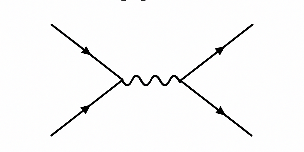
Note. In a Feynman diagram:

Straight lines with arrows represent fermions (e.g., electrons or positrons).

Arrow pointing forward in time: electron.

Arrow pointing backward in time: positron.

Wavy lines represent photons (or, more generally, gauge bosons).

Vertices are interaction points, where lines meet.

In QED, each vertex corresponds to a factor $-ie\gamma^{\mu}$ , representing the electron–photon coupling.

8.3.5 Effective action and 1PI: the grown-up organizing principle

Define the classical field (a.k.a. mean field)

\phi_{c}(x) \equiv \frac{\delta W[J]}{\delta J(x)}

Legendre transform to the effective action

\Gamma[\phi_{c}] \equiv W[J] - \int d^{4}x\,J(x)\,\phi_{c}(x)

with $J$ chosen to produce the given $\phi_{c}$ . Then

\frac{\delta \Gamma}{\delta \phi_{c}(x)} = -\,J(x)

Setting $J=0$ gives the quantum equations of motion $\delta\Gamma/\delta\phi_{c}=0$ . Functional derivatives of $\Gamma$ at a constant background generate 1PI (one-particle irreducible) vertices; expanding $\Gamma$ in loops is the systematic semiclassical expansion.

8.3.6 Schwinger–Dyson equations: integration by parts in field space

Because total functional derivatives vanish under the integral,

\int \mathcal D\phi\;\frac{\delta}{\delta \phi(x)}\left[\,\mathcal F[\phi]\;e^{iS[\phi]}\right] = 0

Choosing $\mathcal F=\phi(y)$ for the scalar theory yields

\left\langle \left(\Box_{x} + m^{2}\right)\phi(x) + \frac{\lambda}{3!}\phi^{3}(x)\right\rangle = -\,i\,\delta^{(4)}(x-y)

and, more generally, a hierarchy that relates $n$ -point to $(n\!+\!1)$ -point functions. In momentum space these become exact integral equations for full propagators/vertices.

8.3.7 Wick rotation: Euclid speedrun

Real-time integrals oscillate; numerics cry. Rotate to Euclidean time $t\to -i\tau$ :

S_{E}[\phi] = \int d^{4}x_{E}\left[\frac{1}{2}(\partial_{\mu}\phi)^{2} + \frac{1}{2}m^{2}\phi^{2} + \frac{\lambda}{4!}\phi^{4}\right]

The weight becomes $e^{-S_{E}}$ and

Z_{E}[J] = \int \mathcal D\phi\;\exp\!\left[-\,S_{E}[\phi] + \int d^{4}x_{E}\,J\phi\right]

Now $Z_{E}$ looks like a statistical partition function. This is the gateway to lattice QFT, Monte-Carlo sampling, and the cluster of ideas linking QFT and critical phenomena. Analytic continuation brings results back to Minkowski.

8.3.8 Gauge fields in the path integral: fixing and ghosts (quick tour)

For gauge fields $A_{\mu}$ , naive

Z = \int \mathcal D A\;e^{iS[A]}

overcounts physically equivalent configurations. Insert a gauge-fixing delta and the Faddeev–Popov determinant:

Z = \int \mathcal D A\,\mathcal D\bar c\,\mathcal D c\;\exp\!\left\{iS[A] + iS_{\text{gf}}[A] + iS_{\text{FP}}[\bar c,c,A]\right\}

In covariant gauges,

S_{\text{gf}} = -\,\frac{1}{2\xi}\int d^{4}x\,(\partial_{\mu}A^{\mu})^{2}

and the ghost action arises from the determinant. A hidden global symmetry—BRST—organizes the bookkeeping and implies Ward/Slavnov–Taylor identities that protect gauge invariance after quantization.

8.3.9 Renormalization and regularization in this language

Loop integrals diverge; regulate (cutoff, dimensional regularization, Pauli–Villars), then renormalize by adding counterterms to $S$ so that physical $n$ -point functions match experiments. The path-integral view makes it clear:

Counterterms are just extra local pieces in the action
Renormalization group tracks how the effective action changes with scale
Anomalies (like the chiral anomaly) appear as non-invariance of the measure under certain transformations (Fujikawa method)

8.3.10 What the pictures mean: rules from $Z[J]$

Disconnected vs connected. $Z$ generates everything; $W=-i\ln Z$ kills disconnected pieces
Amputated vs 1PI. Differentiate $W$ then amputate external propagators to get scattering kernels; differentiate $\Gamma$ to get 1PI vertices directly
Symmetry factors. They’re the combinatorics of repeated derivatives acting on the same source factors—the $1/S$ in front of diagrams

8.3.11 Worked mini-examples

(a) Free Gaussian check.
Show directly from $Z_{0}[J]$ that

G^{(2)}(x,y) = \Delta_{F}(x-y),\qquad G^{(4)}(x_{1},\dots,x_{4}) = \Delta_{12}\Delta_{34} + \Delta_{13}\Delta_{24} + \Delta_{14}\Delta_{23}

with $\Delta_{ij}\equiv \Delta_{F}(x_{i}-x_{j})$ .

(b) Zero-dimensional $\phi^{4}$ (toy model).
Replace $\int \mathcal D\phi$ by $\int d\phi$ for

Z(J) = \int_{-\infty}^{\infty} d\phi\;\exp\!\left[i\left(\frac{1}{2}m^{2}\phi^{2} - \frac{\lambda}{4!}\phi^{4} + J\phi\right)\right]

Expand in $\lambda$ and match to the Feynman-diagram series—no spacetime, all combinatorics.

(c) One-loop tadpole skeleton in $\phi^{4}$ .
From the operator expansion $\exp[-i(\lambda/4!)\int (\delta/i\delta J)^{4}]$ , the $O(\lambda)$ correction to $G^{(2)}$ includes

\frac{-i\lambda}{2}\,\Delta_{F}(x-y)\,\Delta_{F}(0)

exhibiting a UV divergence in $\Delta_{F}(0)$ and motivating mass renormalization.

(d) Classical limit via stationary phase.
Scale $S\to S/\hbar$ and send $\hbar\to 0$ ; the dominant contribution to $Z$ comes from fields solving $\delta S/\delta\phi=0$ with fluctuations generating the loop expansion. This is the precise sense in which “loops are quantum.”

(e) Ward identity from a change of variables.
For a global symmetry $\phi\to \phi + \epsilon\,\delta\phi$ , invariance of the measure and action implies

\int d^{4}x\;\left\langle \partial_{\mu}J^{\mu}(x)\;\mathcal O[\phi]\right\rangle = i\sum_{j}\delta(x-x_{j})\left\langle \frac{\delta \mathcal O}{\delta \phi(x_{j})}\right\rangle

the functional version of current conservation inside correlators.

8.3.12 Minimal problem kit

Derive $Z_{0}[J]$ by completing the square and fix the normalization by demanding $Z_{0}[0]=1$
Starting from $Z[J]$ for $\phi^{4}$ , obtain the momentum-space Feynman rules and identify the symmetry factor for the one-loop “fish” diagram in the 4-point function
Compute the connected two-point function as $\delta^{2}W/\delta J \delta J$ and confirm that $W=-i\ln Z$ removes disconnected pieces
Perform the Wick rotation carefully for $\phi^{4}$ , showing that $iS\to -S_{E}$ and $Z\to Z_{E}$ , and identify how propagators change
Write the Schwinger–Dyson equation for the full propagator $G(x,y)$ in $\phi^{4}$ and express it diagrammatically
For a $U(1)$ gauge theory, sketch the Faddeev–Popov procedure leading to ghosts in covariant gauges and write the BRST transformations

8.4 LSZ Reduction and Scattering Amplitudes

Green’s functions are great for theory; experiments ask for cross sections. The bridge is the LSZ reduction formula: amputate external propagators of time-ordered correlators, put external legs on shell, and you get the $S$ -matrix amplitude $\mathcal M$ . This section lays out LSZ for scalars and fermions, how $Z$ enters, phase space and cross sections, and a few quick examples plus unitarity via the optical theorem.

8.4.1 From correlators to amplitudes: the vibe

Correlators: $G^{(n)} = \langle 0|T\{\phi\cdots\phi\}|0\rangle$
Connected pieces: $W=-i\ln Z$
Amputation: remove external propagators
On-shell limit: $p^{2}\to m^{2}$ (or $/\!\!p\to m$ for fermions)
Wavefunction renormalization: residues of single-particle poles define $Z$ factors

The output is $\mathcal M$ (the thing that goes under $|\mathcal M|^{2}$ in cross sections).

8.4.2 Pole, residue, and the $Z$ factor

For a real scalar field, the full two-point function in momentum space behaves near the one-particle pole as

\tilde G^{(2)}(p) = \int d^{4}x\,e^{ip\cdot x}\,G^{(2)}(x) \;\sim\; \frac{i\,Z_{\phi}}{p^{2}-m^{2}+i\epsilon} + \text{regular}

The residue $Z_{\phi}$ is the probability to create the one-particle state from the field. External legs therefore contribute $Z_{\phi}^{-1/2}$ each in LSZ.

For a Dirac field, similarly

\tilde S(p) \equiv \int d^{4}x\,e^{ip\cdot x}\,\langle 0|T\{\psi(x)\bar\psi(0)\}|0\rangle \;\sim\; \frac{i\,Z_{\psi}(/\!\!p+m)}{p^{2}-m^{2}+i\epsilon}

8.4.3 Scalar LSZ reduction (in → out)

Consider an $n\to m$ process of a neutral scalar with mass $m$ . Let $G^{(n+m)}$ be the full time-ordered correlator. The amputated on-shell amplitude is

\mathcal M(\{p\}\to\{p'\}) = \left[\prod_{a=1}^{n} Z_{\phi}^{-1/2}\; i\!\int d^{4}x_{a}\;e^{ip_{a}\cdot x_{a}}\left(\Box_{x_{a}}+m^{2}\right)\right] \left[\prod_{b=1}^{m} Z_{\phi}^{-1/2}\; i\!\int d^{4}y_{b}\;e^{-ip'_{b}\cdot y_{b}}\left(\Box_{y_{b}}+m^{2}\right)\right] \,G^{(n+m)}(\{x\};\{y\})

All external momenta are taken on shell after differentiations, $p_{a}^{2}=m^{2}$ and $(p'_{b})^{2}=m^{2}$ . Momentum conservation appears as the overall $(2\pi)^{4}\delta^{(4)}(\sum p-\sum p')$ when you Fourier transform.

8.4.4 Fermionic LSZ (with spinors)

For incoming fermions and outgoing antifermions you project with spinors and use Dirac operators. Schematic form for one incoming fermion of momentum $p$ and one outgoing fermion of momentum $p'$ :

\mathcal M \;\propto\; Z_{\psi}^{-1/2}\, \bar u(p') \left[ -i\!\int d^{4}y\,e^{-ip'\cdot y}\,\left(i\overleftarrow{/\!\!partial}_{y}+m\right)\right] \,\langle 0|T\{\psi(y)\cdots\bar\psi(x)\}|0\rangle\, \left[i\!\int d^{4}x\,e^{ip\cdot x}\,\left(i/\!\!partial_{x}-m\right)\right] Z_{\psi}^{-1/2}\, u(p)

Applying all external operators and taking on-shell limits reproduces the standard Feynman-rule amplitude. For external antifermions, replace $u\leftrightarrow v$ and $\psi\leftrightarrow \bar\psi$ projections accordingly.

8.4.5 Why “amputated connected Green functions” matter

Connected: $W=-i\ln Z$ drops disconnected pieces so you do not double-count spectators
Amputated: dividing by external propagators yields kernels that go straight into $\mathcal M$
1PI vs connected: 1PI vertices from $\Gamma[\phi_{c}]$ build connected amputated functions by gluing with full propagators

This is the algebra behind “draw diagrams, attach external legs, evaluate.”

8.4.6 Plane waves, wave packets, and the $i\epsilon$

Strictly, LSZ uses wave packets so overlap integrals converge and switching on/off the interaction adiabatically is meaningful. In practice we compute with plane waves and the $i\epsilon$ prescription keeps causality and the poles on the right side.

8.4.7 Phase space, cross sections, and decay rates

For $n_{i}\to n_{f}$ scattering, define the Lorentz-invariant $n$ -body phase space

d\Pi_{n_{f}}(P;\{p_{f}\}) = \left[\prod_{k=1}^{n_{f}} \frac{d^{3}\mathbf p_{k}}{(2\pi)^{3}\,2E_{k}}\right] (2\pi)^{4}\,\delta^{(4)}\!\left(P-\sum_{k} p_{k}\right)

Two-body scattering in the center-of-mass has flux factor

\mathcal F = 4\sqrt{(p_{1}\cdot p_{2})^{2} - m_{1}^{2}m_{2}^{2}}

and the differential cross section

d\sigma = \frac{|\mathcal M|^{2}}{\mathcal F}\; d\Pi_{n_{f}}

For a decay of a particle with mass $M$ and total momentum $P$ , the width is

d\Gamma = \frac{|\mathcal M|^{2}}{2M}\; d\Pi_{n_{f}}(P;\{p_{f}\})

Spin sums and averages over initial polarizations are applied to $|\mathcal M|^{2}$ as needed.

8.4.8 Unitarity and the optical theorem

$S = 1 + iT$ with $S^{\dagger}S=\mathbb I$ implies

2\,\mathrm{Im}\,\mathcal M_{i\to i} = \sum_{X}\int d\Pi_{X}\; |\mathcal M_{i\to X}|^{2}

The imaginary part of the forward amplitude equals the total cross section (Cutkosky rules cut loops to enforce this at diagram level).

8.4.9 Crossing symmetry (analytic continuation 101)

Because amplitudes are boundary values of analytic functions, moving a particle from initial to final state corresponds to $p\to -p$ continuation. One and the same $\mathcal M$ encodes $s$ , $t$ , $u$ channels—different physical processes are just different kinematic regions.

8.4.10 Quick examples

(a) $\phi^{4}$ , $2\to 2$ at tree level

With interaction $\mathcal L_{\text{int}}=-\lambda\phi^{4}/4!$ and properly normalized external legs,

\mathcal M_{\text{tree}}(2\to 2) = -\,i\lambda

No momentum dependence at tree level; one-loop adds $s,t,u$ logarithms and counterterms.

(b) Yukawa exchange, $f\bar f\to f\bar f$ at tree level

For $\mathcal L_{\text{int}}=-g\,\bar\psi\psi\,\phi$ , the $t$ -channel scalar exchange gives

\mathcal M = (-ig)^{2}\;\bar u(p_{3})u(p_{1})\;\frac{i}{t-m_{\phi}^{2}+i\epsilon}\;\bar v(p_{2})v(p_{4})

with $t=(p_{3}-p_{1})^{2}$ . Spin sums convert the bilinears to traces.

(c) QED current conservation on external legs

For a photon attached to a fermion line,

q_{\mu}\,\bar u(p')\gamma^{\mu}u(p)=0

on shell, so longitudinal polarization drops out of any tree amplitude (Ward identity).

8.4.11 Practical normalizations and factors you will forget once

Each external scalar leg contributes a factor $Z_{\phi}^{-1/2}$ ; each external spinor contributes $Z_{\psi}^{-1/2}$ and a spinor wavefunction $u$ or $v$
Internal lines always use full propagators if you are beyond tree level
Average over initial spin/polarization states, sum over final ones
Identical-particle factors in phase space: divide by $n!$ for $n$ identical final bosons

8.4.12 Caveats: massless quanta and IR

For theories with massless gauge bosons, LSZ of strict Fock states needs care. Soft and collinear radiation make exclusive probabilities IR-divergent; inclusive rates (KLN theorem) are finite. Practically: add soft emission below detector resolution and virtual corrections together.

8.4.13 Worked mini-examples

(1) Derive scalar LSZ from the pole structure.
Start from the Fourier transform of $G^{(n+m)}$ , isolate single-particle poles, read off residues $Z_{\phi}$ , and show that acting with $(\Box+m^{2})$ amputates an external propagator.

(2) Cross section for contact $\phi^{4}$ scattering.
In the CM frame with identical masses $m$ and $|\mathcal M|^{2}=\lambda^{2}$ ,

\frac{d\sigma}{d\Omega} = \frac{\lambda^{2}}{64\pi^{2}s}\,\frac{|\mathbf p_{f}|}{|\mathbf p_{i}|}

with $s=(p_{1}+p_{2})^{2}$ and equal masses giving $|\mathbf p_{f}|=|\mathbf p_{i}|$ .

(3) Optical theorem check in $\phi^{4}$ at one loop.
Take the $s$ -channel bubble; its imaginary part above threshold equals the $2\to 2$ phase-space integral of the tree-level amplitude squared.

(4) Fermion LSZ projector.
Show that inserting $(i\overleftarrow{/\!\!partial}+m)$ on an outgoing $\psi$ line and contracting with $\bar u(p')$ reproduces the usual external spinor factor when $p'^{2}=m^{2}$ .

8.4.14 Minimal problem kit

Starting from the exact two-point function, prove that $Z_{\phi}^{-1/2}(\Box+m^{2})G^{(n+m)}$ amputates one scalar leg and iterate to $n+m$ legs
Write the LSZ formula for $e^{-}\mu^{-}\to e^{-}\mu^{-}$ and recover the standard QED tree amplitude using propagators and vertices
Derive the two-body phase-space element $d\Pi_{2}$ in the CM frame and integrate to get the textbook $2\to 2$ total cross section for a constant $\mathcal M$
Use Cutkosky rules to compute $\mathrm{Im}\,\mathcal M_{ii}$ for a simple one-loop diagram and verify the optical theorem
Show explicitly how crossing maps the $\phi^{4}$ $2\to 2$ amplitude between $s$ , $t$ , and $u$ channels by analytic continuation of external momenta

8.5 Renormalization: Divergences, Counterterms, and the Running of Couplings

Loop diagrams blow up in the ultraviolet. Renormalization is how we tame those infinities, define physical parameters, and predict scale dependence. In this section we do the workflow on the friendly playground of real scalar $\phi^{4}$ in $d=4$ , set up counterterms, regularize with dimensional regularization, extract the $\beta$ function, and write the Callan–Symanzik equation. Moral: couplings run, fields get anomalous dimensions, and predictions depend on a renormalization scale $\mu$ —but observables don’t.

8.5.1 Power counting and what “renormalizable” means

Consider a real scalar with

\mathcal L = \frac{1}{2}(\partial_\mu\phi)(\partial^\mu\phi) - \frac{1}{2}m^{2}\phi^{2} - \frac{\lambda}{4!}\phi^{4}

In $d=4$ , the field has mass dimension $[\phi]=1$ , so $[\lambda]=0$ and $[m^{2}]=2$ . Superficial UV degree of divergence $D$ for a diagram with $L$ loops, $I$ internal lines, and $V_{4}$ quartic vertices is

D = 4L - 2I

Using topological identities, for $\phi^{4}$ one finds that only 2-point and 4-point amplitudes can be primitively divergent in $d=4$ ; higher $n$ -point functions are superficially convergent. That’s “renormalizable” in action.

8.5.2 Counterterm Lagrangian and renormalization conditions

Bare quantities get decorated hats and are split as finite renormalized pieces plus counterterms

\phi_{0} = Z_{\phi}^{1/2}\,\phi,\qquad m_{0}^{2} = m^{2} + \delta m^{2},\qquad \lambda_{0} = \mu^{\epsilon}\,(\lambda + \delta\lambda)

We’ve introduced dimensional regularization with $d=4-\epsilon$ and a scale $\mu$ to keep $\lambda$ dimensionless. The Lagrangian becomes

\mathcal L = \frac{1}{2}Z_{\phi}(\partial\phi)^{2} - \frac{1}{2}(m^{2} + \delta m^{2})\phi^{2} - \frac{1}{4!}(\lambda + \delta\lambda)\phi^{4}

Expanding $Z_{\phi}=1+\delta Z_{\phi}$ yields the counterterm Lagrangian

\mathcal L_{\text{ct}} = \frac{1}{2}\delta Z_{\phi}(\partial\phi)^{2} - \frac{1}{2}\delta m^{2}\phi^{2} - \frac{1}{4!}\delta\lambda\,\phi^{4}

Renormalization conditions fix $\delta Z_{\phi},\delta m^{2},\delta\lambda$ . Two common choices:

On-shell (OS): pole of the exact propagator at $p^{2}=m^{2}$ with residue $1$ and the $4$ -point $1\text{PI}$ at a specified kinematic point equals $\lambda$
Minimal subtraction (MS or $\overline{\text{MS}}$ ): counterterms cancel only the $1/\epsilon$ poles (and some constants in $\overline{\text{MS}}$ ). Fast and scheme-friendly for RG

8.5.3 One-loop: the two-point tadpole and mass renormalization

The $1$ -loop $2$ -point diagram is the tadpole. In dimensional regularization

-i\Sigma_{\text{tad}} = \frac{-i\lambda}{2}\int\!\frac{d^{d}k}{(2\pi)^{d}}\,\frac{i}{k^{2}-m^{2}+i\epsilon}

Evaluating gives

\Sigma_{\text{tad}} = \frac{\lambda m^{2}}{32\pi^{2}}\left(\frac{2}{\epsilon} - \gamma_{E} + \ln 4\pi + \ln\frac{\mu^{2}}{m^{2}} + 1\right) + \text{finite}

In $\overline{\text{MS}}$ we subtract the pole plus the $-\gamma_{E}+\ln 4\pi$ and define $\delta m^{2}$ so that the renormalized self-energy is finite. Note that at one loop $\delta Z_{\phi}=0$ in $\phi^{4}$ ; wavefunction renormalization starts at two loops.

8.5.4 One-loop: the four-point “fish” and coupling renormalization

The $1$ -loop correction to the $4$ -point $1\text{PI}$ comes from the fish in $s,t,u$ channels. At zero external masses or at the symmetric Euclidean point you can isolate the divergence

\Gamma^{(4)}_{\text{1-loop, div}} = -\,\frac{3\lambda^{2}}{16\pi^{2}}\;\frac{1}{\epsilon}

so in $\overline{\text{MS}}$

\delta\lambda = \frac{3\lambda^{2}}{16\pi^{2}}\;\frac{1}{\epsilon}

The factor of $3$ counts $s,t,u$ . Finite pieces depend on kinematics and scheme but do not affect the $\beta$ function at this order.

8.5.5 Renormalization group and the $\beta$ function

Bare parameters do not depend on $\mu$ , so $\mu\,d\lambda_{0}/d\mu=0$ . Using $\lambda_{0}=\mu^{\epsilon}Z_{\lambda}\lambda$ with $Z_{\lambda}=1+\delta\lambda/\lambda$ , define

\beta(\lambda) \equiv \mu\frac{d\lambda}{d\mu}\Big|_{\lambda_{0}} ,\qquad \gamma_{\phi}(\lambda) \equiv \frac{1}{2}\mu\frac{d\ln Z_{\phi}}{d\mu}\Big|_{\lambda_{0}},\qquad \gamma_{m}(\lambda) \equiv \frac{1}{m^{2}}\mu\frac{d m^{2}}{d\mu}\Big|_{\lambda_{0}}

At one loop for real $\phi^{4}$ in $d=4$

\beta(\lambda) = \frac{3}{16\pi^{2}}\lambda^{2}

\gamma_{\phi}(\lambda) = 0 + \mathcal O(\lambda^{2})

\gamma_{m}(\lambda) = \frac{\lambda}{16\pi^{2}} + \mathcal O(\lambda^{2})

Thus $\lambda$ grows with scale in the UV. Solving $d\lambda/d\ln\mu = \frac{3}{16\pi^{2}}\lambda^{2}$ gives

\lambda(\mu) = \frac{\lambda(\mu_{0})}{1 - \dfrac{3\lambda(\mu_{0})}{16\pi^{2}}\ln\!\left(\frac{\mu}{\mu_{0}}\right)}

The denominator can vanish at a finite $\mu$ —the Landau pole—a sign that pure $\phi^{4}$ in $d=4$ is not UV complete by itself.

8.5.6 Callan–Symanzik equation and scaling

An $n$ -point renormalized Green function $G^{(n)}$ satisfies

\left[\mu\frac{\partial}{\partial\mu} + \beta(\lambda)\frac{\partial}{\partial\lambda} - n\,\gamma_{\phi}(\lambda) + \gamma_{m}(\lambda)\,m^{2}\frac{\partial}{\partial m^{2}}\right] G^{(n)}(x_{1},\dots,x_{n};\lambda,m,\mu) = 0

This encodes the statement that physics cannot depend on the arbitrary scale $\mu$ . Solving it resums large logarithms $\ln(p/\mu)$ by running couplings and masses to the relevant scale.

8.5.7 Scheme dependence vs observables

Change renormalization scheme and $\lambda(\mu)$ ’s numeric value shifts, but $S$ -matrix elements and measurable rates are scheme independent when computed consistently to the same order. Popular choices:

On-shell: intuitive but messy beyond one loop
$\overline{\text{MS}}$ : simple poles removed, algebraic cleanroom, default for RG work

You can convert between schemes with finite redefinitions $\lambda \to \lambda + c_{1}\lambda^{2} + \cdots$ .

8.5.8 Anomalous dimensions and field strength

Although $\gamma_{\phi}=0$ at one loop in $\phi^{4}$ , generally fields acquire anomalous dimensions. Correlators then scale with powers corrected by $\gamma_{\phi}$ . In conformal theories at fixed points $\beta=0$ , operator dimensions are classical + anomalous numbers determined by the CFT data.

8.5.9 UV vs IR, logs vs power divergences

Dimensional regularization turns quadratic divergences into poles plus mass dependence, keeping symmetries tidy. UV divergences map to $1/\epsilon$ poles; IR divergences appear as separate poles when masses vanish. Good hygiene:

Use dim reg for gauge theories and RG
Keep an IR regulator when masses are zero and remove it after inclusive observables are formed

8.5.10 Worked mini-examples

(a) Tadpole in $\overline{\text{MS}}$

Show that choosing

\delta m^{2} = \frac{\lambda m^{2}}{32\pi^{2}}\left(\frac{2}{\epsilon}\right)

cancels the UV pole of $\Sigma_{\text{tad}}$ in $\overline{\text{MS}}$ and write the finite leftover self-energy

(b) One-loop $\beta$ from counterterm algebra

Starting from $\lambda_{0}=\mu^{\epsilon}(\lambda+\delta\lambda)$ with $\delta\lambda = \tfrac{3\lambda^{2}}{16\pi^{2}}\tfrac{1}{\epsilon}$ , impose $d\lambda_{0}/d\mu=0$ and derive $\beta(\lambda)=\tfrac{3}{16\pi^{2}}\lambda^{2}$

(c) Running coupling and Landau pole

Given $\lambda(\mu_{0})=0.1$ at $\mu_{0}=m$ , find the scale where the denominator vanishes and interpret physically

(d) Symmetric-point renormalization

Define $\lambda$ by the $1\text{PI}$ $4$ -point at $s=t=u=-\mu^{2}$ . Show that changing $\mu$ shifts $\lambda$ according to the same one-loop $\beta$

(e) Callan–Symanzik for $G^{(2)}$

Write the equation for $G^{(2)}(p^{2})$ in momentum space, use $\gamma_{\phi}=0$ at one loop, and solve the RG-improved propagator to sum leading logs

8.5.11 Minimal problem kit

Perform the one-loop evaluation of the fish diagram with dimensional regularization and extract its pole
Show that $\delta Z_{\phi}=0$ at one loop by inspecting the momentum dependence of the self-energy
Compute $\gamma_{m}$ at one loop from the counterterm $\delta m^{2}$ and verify the result above
Starting from the CS equation, show that $n$ -point functions at large momenta are governed by running couplings evaluated at the hard scale
Compare OS and $\overline{\text{MS}}$ definitions of $\lambda$ at one loop and derive the finite conversion

8.6 Non-Abelian Gauge Fields and Yang–Mills Theory

Electromagnetism is an Abelian $U(1)$ gauge theory: fields don’t talk to each other. The Standard Model runs on non-Abelian gauge symmetry, where the gauge bosons carry charge and self-interact. This section builds Yang–Mills (YM) theory, couples it to matter, quantizes with gauge fixing and ghosts, and sketches BRST symmetry, Wilson lines, and the one-loop $\beta$ function behind asymptotic freedom.

Standard Model

8.6.1 Gauge groups, generators, and covariant derivatives

Let $G$ be a compact Lie group with generators $T^{a}$ in some representation, satisfying

[T^{a},T^{b}] = i f^{abc} T^{c}

Normalize color algebra by

\mathrm{tr}(T^{a}T^{b}) = T_{R}\,\delta^{ab},\qquad T^{a}T^{a} = C_{F}\,\mathbb I,\qquad f^{acd}f^{bcd} = C_{A}\,\delta^{ab}

For $G=SU(N)$ in the fundamental rep, $T_{R}=\tfrac12$ , $C_{F}=\tfrac{N^{2}-1}{2N}$ , $C_{A}=N$ .

A matter field $\psi$ transforms as $\psi \to U(x)\psi$ with $U(x)\in G$ . The covariant derivative is

D_{\mu} \equiv \partial_{\mu} + i g\,A_{\mu}^{a} T^{a}

so that $D_{\mu}\psi$ transforms like $\psi$ . The non-Abelian field strength comes from the commutator

[D_{\mu},D_{\nu}] = i g\,F_{\mu\nu}^{a} T^{a}

with

F_{\mu\nu}^{a} = \partial_{\mu}A_{\nu}^{a} - \partial_{\nu}A_{\mu}^{a} + g f^{abc} A_{\mu}^{b} A_{\nu}^{c}

8.6.2 Yang–Mills Lagrangian and equations of motion

The YM action with Dirac matter is

\mathcal L_{\mathrm{YM+mat}} = -\,\frac{1}{4}\,F_{\mu\nu}^{a} F^{a\,\mu\nu} + \bar\psi\,(i\gamma^{\mu} D_{\mu} - m)\,\psi

Infinitesimal gauge transformations with parameters $\alpha^{a}(x)$ act as

\delta \psi = i g\,\alpha^{a} T^{a} \psi,\qquad \delta A_{\mu}^{a} = -\,\frac{1}{g}\,(D_{\mu}\alpha)^{a}

The YM equations of motion are

(D_{\mu} F^{\mu\nu})^{a} = g\,\bar\psi\,\gamma^{\nu} T^{a}\psi

plus the Bianchi identity $D_{[\mu}F_{\nu\rho]}=0$ .

Three- and four-gluon interactions. Expanding $F^{2}$ shows cubic $\sim g f^{abc}(\partial A)AA$ and quartic $\sim g^{2} f^{abe} f^{cde} A^{a}A^{b}A^{c}A^{d}$ self-interactions, absent in QED.

8.6.3 Gauge fixing, ghosts, and propagators

Path integrating over $A_{\mu}$ overcounts gauge copies. In covariant gauges add

\mathcal L_{\mathrm{gf}} = -\,\frac{1}{2\xi}\,(\partial_{\mu}A^{a\,\mu})^{2}

and Faddeev–Popov ghost fields $c^{a},\bar c^{a}$ with

\mathcal L_{\mathrm{FP}} = (\partial_{\mu}\bar c^{a})\,(D^{\mu} c)^{a}

Ghosts are anticommuting scalars that only run in loops. In momentum space the gluon propagator is

\tilde D_{\mu\nu}^{ab}(k) = \frac{-\,i\,\delta^{ab}}{k^{2}+i\epsilon}\left[g_{\mu\nu} - (1-\xi)\frac{k_{\mu}k_{\nu}}{k^{2}}\right]

and the ghost propagator is $i\,\delta^{ab}/(k^{2}+i\epsilon)$ . Feynman gauge is $\xi=1$ , Landau gauge is $\xi=0$ .

8.6.4 BRST symmetry in one screen

Gauge fixing breaks gauge symmetry but leaves a rigid BRST invariance generated by a nilpotent differential $s$ :

s\,A_{\mu}^{a} = (D_{\mu} c)^{a},\qquad s\,c^{a} = -\,\frac{g}{2}\,f^{abc} c^{b} c^{c},\qquad s\,\bar c^{a} = \frac{1}{\xi}\,\partial_{\mu}A^{a\,\mu},\qquad s\,\psi = i g\,c^{a} T^{a}\psi

with $s^{2}=0$ on all fields. The gauge-fixed action $\mathcal L_{\mathrm{YM}}+\mathcal L_{\mathrm{gf}}+\mathcal L_{\mathrm{FP}}$ is BRST invariant. Physical states live in the BRST cohomology (closed but not exact), which enforces decoupling of unphysical polarizations and ghosts.

8.6.5 Feynman rules and color factors

Vertex list (momenta all incoming):

Gluon–gluon–gluon
Vertex $-g f^{abc}\,[g^{\mu\nu}(k-p)^{\rho} + g^{\nu\rho}(p-q)^{\mu} + g^{\rho\mu}(q-k)^{\nu}]$
Four-gluon
$-i g^{2}\big[f^{abe}f^{cde}(g^{\mu\rho}g^{\nu\sigma}-g^{\mu\sigma}g^{\nu\rho}) + \text{cyclic}\big]$
Gluon–ghost–ghost
$-g f^{abc}\,k_{\mu}$ where $k$ flows from ghost to anti-ghost into the vertex
Gluon–fermion–fermion
$-i g\,\gamma^{\mu} T^{a}$

Color algebra shortcuts:

T^{a}_{ij} T^{a}_{kl} = T_{R}\left(\delta_{il}\delta_{jk} - \frac{1}{N}\delta_{ij}\delta_{kl}\right)\quad\text{for}\ SU(N)

and

\sum_{a} (T^{a}T^{a})_{ij} = C_{F}\,\delta_{ij}

These appear when squaring amplitudes and summing colors.

8.6.6 Wilson lines, loops, and gauge-invariant observables

Parallel transport along a path $\mathcal C$ uses the Wilson line

W(\mathcal C) = \mathcal P \exp\!\left(i g \int_{\mathcal C} A_{\mu}^{a} T^{a}\,dx^{\mu}\right)

Closed loops $\mathrm{tr}\,W(\mathcal C)$ are gauge invariant. In nonperturbative regimes, the area vs perimeter law of large rectangular loops diagnoses confinement. In perturbation theory, Wilson lines resum soft gluon effects.

8.6.7 Beta function and asymptotic freedom

At one loop, with $n_{f}$ Dirac fermions and $n_{s}$ complex scalars in the fundamental representation,

\beta(g) \equiv \mu\,\frac{dg}{d\mu} = -\,\frac{g^{3}}{16\pi^{2}}\left(\frac{11}{3}C_{A} - \frac{4}{3}T_{R} n_{f} - \frac{1}{6} T_{R} n_{s}\right)

For QCD ( $SU(3)$ , $T_{R}=\tfrac12$ , $n_{s}=0$ ),

\beta(g) = -\,\frac{g^{3}}{16\pi^{2}}\left(11 - \frac{2}{3}n_{f}\right)

Negative $\beta$ means the coupling decreases at high scales (asymptotic freedom) if $n_{f} < 17$ for $SU(3)$ . Conversely, it grows in the IR, hinting at confinement.

8.6.8 Topological term and $CP$

Besides $-\tfrac14 F^{2}$ , the Lorentz- and gauge-invariant density

\mathcal L_{\theta} = \theta\,\frac{g^{2}}{32\pi^{2}}\,F_{\mu\nu}^{a}\,\tilde F^{a\,\mu\nu},\qquad \tilde F^{\mu\nu} \equiv \frac{1}{2}\,\epsilon^{\mu\nu\rho\sigma} F_{\rho\sigma}

is a total derivative classically but affects quantum physics via nontrivial gauge bundles. It is odd under $CP$ and $T$ , even under $C$ and $P$ separately only for Abelian cases. We return to anomalies and topology in §8.10.

8.6.9 Worked mini-examples

(a) Derive the three-gluon vertex.
Expand $-\tfrac14 F^{a}_{\mu\nu}F^{a\,\mu\nu}$ keeping terms cubic in $A$ and read off the momentum-space rule.

(b) Color factors in $q\bar q\to q'\bar q'$ .
Show that averaging over incoming colors yields an overall $T_{R}^{2}$ and a $C_{F}$ trace on the fermion line.

(c) Ghost loop in the gluon self-energy.
Compute the sign and tensor structure; confirm that the sum of gluon and ghost loops is transverse, $k_{\mu}\Pi^{\mu\nu}(k)=0$ .

(d) BRST nilpotency on $A_{\mu}$ .
Use $s A_{\mu}^{a}=(D_{\mu}c)^{a}$ and $s c^{a}=-\tfrac{g}{2} f^{abc} c^{b}c^{c}$ to show $s^{2}A_{\mu}^{a}=0$ via the Jacobi identity.

(e) One-loop $\beta$ sign.
Count diagrams contributing to the gluon two-point: gluon loop $\propto +\tfrac{11}{3}C_{A}$ , fermion loop $\propto -\tfrac{4}{3}T_{R} n_{f}$ , scalar loop $\propto -\tfrac{1}{6}T_{R} n_{s}$ and combine.

8.6.10 Minimal problem kit

Starting from $D_{\mu}$ , derive $F_{\mu\nu}$ and prove the Bianchi identity $D_{[\mu}F_{\nu\rho]}=0$
Quantize YM in covariant gauge and write the complete Feynman rules including ghosts
Show that the Slavnov–Taylor identity enforces transversality of the renormalized gluon propagator and charge universality at a quark–gluon vertex
Compute the Wilson loop at order $g^{2}$ around a rectangle and interpret the Coulomb potential from its logarithm
Derive the one-loop $\beta$ function using background-field gauge to keep manifest gauge invariance of the effective action

8.7 QED in Practice: Core Processes, One-Loop Signatures, and the Running of $\alpha$

QED is the clean room of particle physics: an exactly tested gauge theory where symmetry wins arguments and numbers match 12+ digits. This section puts the tools to work—tree-level scattering, how infrared safety actually happens, what one-loop does (vacuum polarization, vertex correction, electron self-energy), and why the electric charge runs with scale.

Conventions: natural units ( $\hbar=c=1$ ). Metric $g_{\mu\nu}=\mathrm{diag}(+,-,-,-)$ . Electron charge $e>0$ so the electron has $-e$ . Fine-structure constant $\alpha\equiv e^{2}/4\pi$ .

8.7.1 Lagrangian, fields, and Ward identities (reminder)

The QED Lagrangian is

\mathcal L_{\mathrm{QED}}=\bar\psi(i\gamma^{\mu}D_{\mu}-m)\psi - \frac{1}{4}F_{\mu\nu}F^{\mu\nu},\qquad D_{\mu}=\partial_{\mu}+ieA_{\mu}

Gauge invariance $\psi\to e^{i\alpha(x)}\psi$ , $A_{\mu}\to A_{\mu}-\partial_{\mu}\alpha/e$ implies current conservation and the Ward–Takahashi identity

q_{\mu}\,\Gamma^{\mu}(p',p) = S^{-1}(p') - S^{-1}(p)

which enforces $Z_{1}=Z_{2}$ (vertex and wavefunction renormalizations equal) and kills longitudinal photon pieces in amplitudes.

8.7.2 Feynman rules you actually use

Fermion propagator: $i(/\!\! p + m)/(p^{2}-m^{2}+i\epsilon)$
Photon propagator (covariant gauge):

\frac{-i}{k^{2}+i\epsilon}\left[g_{\mu\nu} - (1-\xi)\frac{k_{\mu}k_{\nu}}{k^{2}}\right]

Vertex: $-ie\gamma^{\mu}$
External lines: $u,\bar u,v,\bar v$ spinors; photon polarization $\epsilon^{\mu}$ with $q\cdot\epsilon=0$ in physical gauges

8.7.3 Textbook tree: $e^{+}e^{-}\to \mu^{+}\mu^{-}$

One $s$ -channel photon:

\mathcal M = \bar v(p_{2})\,(-ie\gamma^{\mu})\,u(p_{1})\;\frac{-i g_{\mu\nu}}{s}\;\bar u(k_{1})\,(-ie\gamma^{\nu})\,v(k_{2})

CM frame with $m_{e},m_{\mu}\approx 0$ gives

\overline{|\mathcal M|^{2}} = 2 e^{4}\,(1+\cos^{2}\theta)

and differential cross section

\frac{d\sigma}{d\Omega} = \frac{\alpha^{2}}{4s}\,(1+\cos^{2}\theta)

Total cross section

\sigma(e^{+}e^{-}\to \mu^{+}\mu^{-}) = \frac{4\pi\alpha^{2}}{3s}

This is the R-ratio baseline used to see quark thresholds when you replace $\mu$ by $\sum_{q}Q_{q}^{2}$ times color.

8.7.4 Bhabha and Møller: identical charges and $t$ -channel spice

Bhabha ( $e^{+}e^{-}\to e^{+}e^{-}$ ): $s$ -channel $+$ $t$ -channel interfere. At small angles the $t$ -channel dominates $\sim 1/\theta^{4}$ , used for luminosity monitoring.
Møller ( $e^{-}e^{-}\to e^{-}e^{-}$ ): $t$ and $u$ with minus signs from Fermi statistics; forward peaking again.

Both are masterclasses in spinor traces and interference. Remember to average/ sum spins and mind identical-particle $1/2!$ when relevant.

8.7.5 Compton scattering: $e\gamma\to e\gamma$

Two diagrams (s- and u-channel). Klein–Nishina formula emerges after spin sums. In the electron rest frame with incoming photon energy $\omega$ and scattering angle $\theta$ ,

\frac{d\sigma}{d\Omega} = \frac{r_{e}^{2}}{2}\left(\frac{\omega'}{\omega}\right)^{2}\left(\frac{\omega'}{\omega}+\frac{\omega}{\omega'}-\sin^{2}\theta\right)

with classical radius $r_{e}=e^{2}/4\pi m$ and

\omega' = \frac{\omega}{1+\frac{\omega}{m}(1-\cos\theta)}

Low-energy limit $\omega\ll m$ gives Thomson scattering $d\sigma/d\Omega = r_{e}^{2}(1+\cos^{2}\theta)/2$ .

8.7.6 Mott scattering: electrons off a Coulomb field

Scattering off an external charge $Z$ via one-photon exchange yields the Mott cross section

\left(\frac{d\sigma}{d\Omega}\right)_{\mathrm{Mott}} = \left(\frac{Z\alpha}{2p\sin^{2}\tfrac{\theta}{2}}\right)^{2}\cos^{2}\tfrac{\theta}{2}

Relativistic spin effects appear as the $\cos^{2}\tfrac{\theta}{2}$ factor compared to Rutherford.

8.7.7 Infrared (IR) physics: soft photons and KLN safety

Virtual one-loop diagrams with photons cause IR divergences; so do real emissions with a soft photon of energy $\omega<\Delta E$ . Bloch–Nordsieck/KLN theorem: virtual + real at fixed detector resolution is finite. Skeleton for any $2\to 2$ QED process:

Virtual soft correction $\propto \alpha\,\ln^{2}\!\left(\frac{\lambda}{E}\right)$ or $\alpha\,\ln\!\lambda$ with IR regulator $\lambda$
Real soft emission $\propto -$ same logs with $\lambda\to \Delta E$
Sum: regulator cancels, leftover $\ln(E/\Delta E)$ is physical (depends on what you count as “seen”)

Practical rule: when computing NLO, always add the soft+collinear real photon slice compatible with your measurement.

8.7.8 One-loop self-energies and renormalization snapshots

Electron self-energy $\Sigma(/\!\! p)$ renormalizes mass and wavefunction. In $\overline{\mathrm{MS}}$ at one loop,

\Sigma(\/\!\! p) = \frac{\alpha}{4\pi}\left[\left(\frac{1}{\epsilon}-\gamma_{E}+\ln 4\pi\right)(-/\!\! p + 4m) + \cdots\right]

Vacuum polarization (photon self-energy) has tensor structure

\Pi_{\mu\nu}(q) = \left(q_{\mu}q_{\nu}-q^{2}g_{\mu\nu}\right)\Pi(q^{2})

Gauge invariance forces transversality $q^{\mu}\Pi_{\mu\nu}=0$ . At one loop with a fermion of mass $m$ ,

\Pi(q^{2}) = \frac{\alpha}{3\pi}\left(\frac{1}{\epsilon}-\gamma_{E}+\ln 4\pi - \ln\frac{m^{2}}{\mu^{2}}\right) + \text{finite}(q^{2}/m^{2})

Vertex correction $\Gamma^{\mu}=\gamma^{\mu}F_{1}(q^{2}) + \frac{i\sigma^{\mu\nu}q_{\nu}}{2m}F_{2}(q^{2})$ generates the anomalous magnetic moment $a_{e}=F_{2}(0)$ .

At one loop (Schwinger):

a_{e} = \frac{\alpha}{2\pi}

Higher loops keep adding tiny digits that experiments keep confirming.

8.7.9 Running of the electromagnetic coupling

Vacuum polarization dresses the photon and makes the effective charge scale-dependent. Define

\alpha(q^{2}) = \frac{\alpha(\mu^{2})}{1 - \Delta\alpha(q^{2},\mu^{2})}

At leading order for a fermion of charge $Q_{f}$ and mass $m_{f}$ ,

\Delta\alpha(q^{2},\mu^{2}) = \frac{\alpha}{3\pi}\,Q_{f}^{2}\,\ln\!\left(\frac{q^{2}}{\mu^{2}}\right) + \cdots

Summing all charged species up to the scale increases $\alpha$ mildly: from $\alpha^{-1}\approx 137$ at $q^{2}\approx 0$ to $\alpha^{-1}\approx 128$ near the $Z$ pole (numbers for intuition; details depend on hadronic vacuum polarization).

8.7.10 Polarization sums, gauge choices, and sanity checks

For internal photons in covariant gauges, keep the full propagator; Ward identities guarantee $\xi$ cancels in observables
For external real photons, you can use

\sum_{\lambda}\epsilon_{\mu}^{(\lambda)}(q)\,\epsilon_{\nu}^{(\lambda)\ast}(q) = -g_{\mu\nu}

after proving $q_{\mu}\mathcal M^{\mu}=0$ for each coupling current

For spin sums, standard traces:

\sum_{s}u^{s}(p)\bar u^{s}(p)=/\!\! p+m,\qquad \sum_{s}v^{s}(p)\bar v^{s}(p)=/\!\! p-m

8.7.11 Worked mini-examples

(a) $e^{+}e^{-}\to \mu^{+}\mu^{-}$ trace drill
Evaluate $\overline{|\mathcal M|^{2}}$ using traces of $\gamma$ matrices and confirm $(1+\cos^{2}\theta)$ .

(b) Soft photon factorization
Show that in the soft limit the $n\to m+\gamma_{\mathrm{soft}}$ amplitude factorizes:

\mathcal M_{\mathrm{soft}} = \mathcal M_{0}\;\left[e\sum_{i\in\text{charged legs}}\eta_{i}\frac{p_{i}\cdot \epsilon}{p_{i}\cdot q}\right]

with $\eta_{i}=\pm 1$ for outgoing/incoming charges.

(c) One-loop $a_{e}$ sketch
Project the vertex onto $\sigma^{\mu\nu}$ at $q^{2}\to 0$ and integrate Feynman parameters to get $F_{2}(0)=\alpha/2\pi$ .

(d) Vacuum polarization and $\alpha(q^{2})$
Compute $\Pi(q^{2})$ in the limit $|q^{2}|\gg m^{2}$ and derive the leading logarithm of $\alpha$ ’s running.

(e) Compton low-energy limit
Expand the tree amplitude for $\omega\ll m$ and recover the Thomson cross section.

8.7.12 Minimal problem kit

Derive the Bhabha differential cross section at tree level in the massless limit; identify the $s\leftrightarrow t$ symmetry and small-angle behavior
Compute the Klein–Nishina formula from the two diagrams and show the Thomson limit
Demonstrate the cancellation of the IR regulator between virtual and soft-real contributions for $e^{+}e^{-}\to \mu^{+}\mu^{-}$ at NLO, leaving $\ln(E/\Delta E)$
Using Ward–Takahashi, prove $Z_{1}=Z_{2}$ at one loop in dimensional regularization
From the renormalized photon propagator, extract the effective charge in the Thomson limit and near a heavy-fermion threshold; discuss decoupling vs matching

8.8 Spontaneous Symmetry Breaking: Goldstone and Higgs Mechanisms

Sometimes the equations have more symmetry than the ground state chooses to show off. That mismatch is spontaneous symmetry breaking (SSB). In global theories it yields massless Goldstone bosons; in gauge theories those would-be Goldstones get eaten, giving mass to gauge bosons via the Higgs mechanism. This section does the global $U(1)$ story, the Abelian Higgs model, the non-Abelian generalization, and a sneak peek at the electroweak sector. We also hit effective potentials and a quick tour of topological defects.

8.8.1 What “spontaneous” means

The Lagrangian has a continuous symmetry, but the vacuum does not. There are degenerate minima related by the symmetry, and the theory “picks one,” breaking it. The excitations along the flat directions are Goldstones; transverse ones are massive.

Order parameter: a field or composite whose vacuum expectation value (vev) is not invariant under the symmetry. We denote it by $v$ .

8.8.2 Global $U(1)$ with a complex scalar: Mexican hat 101

Consider a single complex scalar $\phi$ with a global $U(1)$ symmetry $\phi\to e^{i\alpha}\phi$ and

\mathcal L = \partial_{\mu}\phi^{\ast}\partial^{\mu}\phi - V(\phi),\qquad V(\phi) = -\,\mu^{2}\,|\phi|^{2} + \frac{\lambda}{2}\,|\phi|^{4},\quad \mu^{2}>0,\ \lambda>0

The minima satisfy $|\phi|^{2}=v^{2}/2$ with

v \equiv \sqrt{\frac{2\mu^{2}}{\lambda}}

Pick one vacuum and expand

\phi(x) = \frac{1}{\sqrt{2}}\,[v + h(x) + i\,\pi(x)]

Plug in and keep quadratic terms

\mathcal L_{\text{quad}} = \frac{1}{2}(\partial h)^{2} + \frac{1}{2}(\partial \pi)^{2} - \frac{1}{2}\,m_{h}^{2}\,h^{2}

with

m_{h}^{2} = \lambda v^{2},\qquad m_{\pi}^{2} = 0

So $h$ is a massive radial mode and $\pi$ is a massless Goldstone boson from breaking $U(1)\to \{\}$

8.8.3 Goldstone’s theorem in one screen

For a continuous global symmetry with conserved current $J^{\mu}_{a}$ and charge $Q_{a}$ , if some local operator $\mathcal O$ has a vev that is not invariant, $\langle 0|[Q_{a},\mathcal O]|0\rangle\neq 0$ , then there exists a massless spin-0 mode. More generally, for Lie group $G$ broken to $H$ , the number of Goldstones equals the number of broken generators

N_{\text{GB}} = \dim G - \dim H

In relativistic theories with Lorentz-invariant vacua, Goldstones have linear dispersion at small momentum

8.8.4 Abelian Higgs mechanism: eating the Goldstone

Now gauge the $U(1)$ with coupling $g$ . Replace $\partial_{\mu}\to D_{\mu}=\partial_{\mu}+igA_{\mu}$

\mathcal L = -\frac{1}{4}F_{\mu\nu}F^{\mu\nu} + |D_{\mu}\phi|^{2} - \left(-\mu^{2}|\phi|^{2} + \frac{\lambda}{2}|\phi|^{4}\right)

Expand around the same vev. In unitary gauge set the phase to zero and write

\phi(x) = \frac{1}{\sqrt{2}}\,[v + h(x)]

The quadratic Lagrangian contains

\mathcal L_{\text{quad}} \supset \frac{1}{2}(\partial h)^{2} - \frac{1}{2}m_{h}^{2}h^{2} + \frac{1}{2}m_{A}^{2}\,A_{\mu}A^{\mu}

with masses

m_{h}^{2} = \lambda v^{2},\qquad m_{A}^{2} = g^{2} v^{2}

Degree-of-freedom audit:

Before SSB: complex scalar $=2$ real d.o.f. plus massless gauge field $=2$ transverse polarizations, total $4$
After SSB: one real scalar $h$ $=1$ plus massive vector $A_{\mu}$ $=3$ polarizations, total $4$

The Goldstone $\pi$ did not vanish; it became the longitudinal polarization of the massive gauge boson

8.8.5 $R_{\xi}$ gauges, would-be Goldstones, and BRST

Unitary gauge hides renormalizability. In covariant $R_{\xi}$ gauges add

\mathcal L_{\text{gf}} = -\,\frac{1}{2\xi}\left(\partial_{\mu}A^{\mu} - \xi\,g\,v\,\pi\right)^{2}

The would-be Goldstone $\pi$ propagates with mass

m_{\pi}^{2} = \xi\,m_{A}^{2}

and Faddeev–Popov ghosts also pick up $\xi$ -dependent masses. Physical observables are $\xi$ -independent; BRST symmetry keeps the cancellations honest

8.8.6 Non-Abelian Higgs mechanism: $G\to H$

Let $\phi$ transform under a representation of a non-Abelian group $G$ , and choose a potential whose minima break $G$ down to a subgroup $H$ . Write the covariant derivative $D_{\mu}=\partial_{\mu}+ig A_{\mu}^{a} T^{a}$ . Expanding about a vev $\langle\phi\rangle$ yields a gauge-boson mass matrix

(M^{2})^{ab} \propto g^{2}\,\langle\phi\rangle^{\dagger}\{T^{a},T^{b}\}\langle\phi\rangle

Gauge bosons corresponding to broken generators acquire masses and eat the corresponding Goldstones; those for unbroken generators remain massless and generate the residual gauge group $H$

8.8.7 Electroweak teaser: $SU(2)_{L}\times U(1)_{Y}\to U(1)_{\text{em}}$

Take a complex scalar doublet $H$ with hypercharge $Y=1/2$ and potential $V=-\mu^{2}H^{\dagger}H+\lambda(H^{\dagger}H)^{2}$ . With

\langle H\rangle = \frac{1}{\sqrt{2}}\begin{pmatrix}0\\ v\end{pmatrix},\qquad v \approx 246\ \text{GeV}

the gauge boson masses are

m_{W} = \frac{g v}{2},\qquad m_{Z} = \frac{\sqrt{g^{2}+g'^{2}}\,v}{2},\qquad m_{\gamma} = 0

The physical scalar $h$ has

m_{h}^{2} = 2\lambda v^{2}

Yukawa couplings $\mathcal L_{Y} = -\,y_{f}\,\bar f_{L} H f_{R} + \text{h.c.}$ give fermion masses

m_{f} = \frac{y_{f} v}{\sqrt{2}}

So couplings to $h$ scale with mass, which is why heavy stuff talks to the Higgs loudly

8.8.8 Effective potential and radiative breaking

Quantum corrections reshape the potential into an effective potential $V_{\text{eff}}(\phi)$ whose minima set the true vacuum

e^{i\int d^{4}x\,\left[-V_{\text{eff}}(\phi_{c})\right]} \sim \int \mathcal D\varphi\ \exp\!\left\{iS[\phi_{c}+\varphi]\right\}

One-loop in $\overline{\text{MS}}$ schematically gives

V_{\text{eff}}^{(1)}(\phi) = \sum_{i}\frac{n_{i}}{64\pi^{2}}\,M_{i}^{4}(\phi)\left[\ln\!\left(\frac{M_{i}^{2}(\phi)}{\mu^{2}}\right) - c_{i}\right]

where $M_{i}(\phi)$ are field-dependent masses and $n_{i}$ counts degrees of freedom with a sign for fermions. Sometimes radiative effects induce SSB even when $\mu^{2}=0$ at tree level (Coleman–Weinberg mechanism)

8.8.9 Topological textures: when vacua have holes

The vacuum manifold $\mathcal M=G/H$ can have nontrivial topology. Defects depend on its homotopy groups

$\pi_{0}(\mathcal M)\neq 0$ → domain walls from discrete breaking
$\pi_{1}(\mathcal M)\neq 0$ → strings; global $U(1)$ gives global strings, gauged $U(1)$ gives Abrikosov–Nielsen–Olesen vortices
$\pi_{2}(\mathcal M)\neq 0$ → monopoles in suitable non-Abelian breakings

These can appear in condensed matter or cosmology and leave measurable footprints

8.8.10 Worked mini-examples

(a) Mass spectrum in Abelian Higgs

Start from $|D\phi|^{2}$ with $\phi=(v+h+i\pi)/\sqrt{2}$ . Expand the kinetic term to show $A_{\mu}$ picks up $\tfrac{1}{2}g^{2}v^{2}A_{\mu}A^{\mu}$ and that the $A_{\mu}\partial^{\mu}\pi$ mixing is removed by the $R_{\xi}$ gauge-fixing choice, leaving $m_{A}^{2}=g^{2}v^{2}$ and $m_{\pi}^{2}=\xi m_{A}^{2}$

(b) Counting Goldstones for $O(N)\to O(N-1)$

Real $N$ -vector $\boldsymbol{\phi}$ with $V=-\tfrac{1}{2}\mu^{2}\boldsymbol{\phi}^{2}+\tfrac{\lambda}{4}(\boldsymbol{\phi}^{2})^{2}$ gives $G/H=O(N)/O(N-1)\cong S^{N-1}$ . Broken generators: $N-1$ Goldstones and one massive radial mode with $m_{h}^{2}=2\lambda v^{2}$

(c) Yukawa masses from the vev

Given $-y\bar\psi_{L}\phi \psi_{R}+\text{h.c.}$ for a complex scalar with $\langle\phi\rangle=v/\sqrt{2}$ , show the fermion mass is $m=yv/\sqrt{2}$ and the physical Higgs coupling is $y=\sqrt{2}m/v$

(d) Non-Abelian mass matrix

For $\phi$ in representation $R$ , derive $(M^{2})^{ab} \propto g^{2}\,\langle\phi\rangle^{\dagger} T^{\{a}T^{b\}} \langle\phi\rangle$ and diagonalize in a simple $SU(2)\to \{\}$ example to find three degenerate massive gauge bosons

(e) One-loop $V_{\text{eff}}$ stationarity

Take a toy spectrum $M_{h}^{2}(\phi)=3\lambda\phi^{2}-\mu^{2}$ , $M_{\pi}^{2}(\phi)=\lambda\phi^{2}-\mu^{2}$ for the global $U(1)$ . Write the stationarity condition $dV_{\text{eff}}/d\phi=0$ and discuss running-coupling improvement by choosing $\mu\sim \phi$

8.8.11 Minimal problem kit

Prove the Goldstone counting $N_{\text{GB}}=\dim G - \dim H$ for a relativistic theory with Lorentz-invariant vacuum
Derive the Abelian Higgs mass spectrum in $R_{\xi}$ gauge and verify $\xi$ -independence of the pole masses
For $SU(2)_{L}\times U(1)_{Y}$ with a single Higgs doublet, derive $m_{W}$ , $m_{Z}$ , and the weak mixing angle relation $\cos\theta_{W}=m_{W}/m_{Z}$
Compute the scattering amplitude $W_{L}W_{L}\to W_{L}W_{L}$ at high energy and show how the Higgs exchange tames the growth with $s$
In a global $U(1)$ model, construct the Noether current and show that the Goldstone couples derivatively, producing suppressed low-energy amplitudes

8.9 Quantum Chromodynamics (QCD): Color, Partons, and Confinement

QCD is the non-Abelian $SU(3)_{\text{color}}$ gauge theory of quarks and gluons. It is weakly coupled at short distances (asymptotic freedom) and strongly coupled at long distances (confinement). The degrees of freedom you scatter in colliders are partons; the stuff you detect are hadrons. The bridge is factorization plus running and a big dose of symmetry.

8.9.1 Lagrangian, fields, and color algebra

With $n_{f}$ quark flavors $\psi_{f}$ in the fundamental of $SU(3)$ and gluons $A_{\mu}^{a}$ in the adjoint, the QCD Lagrangian is

\mathcal L_{\mathrm{QCD}} = -\,\frac{1}{4}\,F_{\mu\nu}^{a} F^{a\,\mu\nu} + \sum_{f=1}^{n_{f}} \bar\psi_{f}\,(i\gamma^{\mu} D_{\mu} - m_{f})\,\psi_{f}

with covariant derivative and field strength

D_{\mu} = \partial_{\mu} + i g\,A_{\mu}^{a} T^{a},\qquad F_{\mu\nu}^{a} = \partial_{\mu}A_{\nu}^{a} - \partial_{\nu}A_{\mu}^{a} + g f^{abc} A_{\mu}^{b} A_{\nu}^{c}

Color factors for $SU(3)$ :

C_{A}=3,\qquad C_{F}=\frac{4}{3},\qquad T_{R}=\frac{1}{2}

These constants run the show in amplitudes, splitting functions, and the $\beta$ function.

8.9.2 Asymptotic freedom and the running coupling

At one loop the QCD $\beta$ function is

\beta(g) \equiv \mu\frac{dg}{d\mu} = -\,\frac{g^{3}}{16\pi^{2}}\left(\frac{11}{3}C_{A} - \frac{4}{3}T_{R} n_{f}\right) + \cdots

For $SU(3)$ this becomes $\beta(g)=-(g^{3}/16\pi^{2})(11 - 2n_{f}/3)$ , which is negative for physical $n_{f}$ . In terms of $\alpha_{s}\equiv g^{2}/4\pi$ ,

\alpha_{s}(\mu) = \frac{4\pi}{\beta_{0}\,\ln(\mu^{2}/\Lambda_{\mathrm{QCD}}^{2})},\qquad \beta_{0}=11 - \frac{2}{3}n_{f}

Coupling shrinks at high $\mu$ (UV freedom) and grows near $\Lambda_{\mathrm{QCD}}$ (IR drama). Across heavy-quark thresholds one matches $n_{f}$ .

8.9.3 Confinement, flux tubes, and hadronization

Nonperturbative QCD appears to confine color: isolated quarks and gluons are not observed. Intuition:

The non-Abelian field lines self-interact and bundle into flux tubes. Long strings cost energy $\propto r$ and eventually snap, creating quark–antiquark pairs
On the lattice, the static quark potential looks like a Cornell shape

V(r) \simeq -\,\frac{4\alpha_{s}}{3\,r} + \kappa r

with a short-distance Coulomb and a long-distance linear rise. In high-energy events, confinement shows up as jets: collimated sprays that remember their parent parton.

8.9.4 Chiral symmetry and its breaking

With light $u,d,s$ quarks and $m_{q}\ll \Lambda_{\mathrm{QCD}}$ , the classical Lagrangian has an approximate global symmetry

SU(N_{f})_{L}\times SU(N_{f})_{R} \to SU(N_{f})_{V}

spontaneously broken by a quark condensate $\langle \bar q q\rangle$ . The resulting Goldstone bosons are the light pseudoscalars; explicit quark masses make them pseudo-Goldstones. The Gell-Mann–Oakes–Renner relation is

f_{\pi}^{2} m_{\pi}^{2} \simeq -\,(m_{u}+m_{d})\,\langle \bar q q \rangle

An axial $U(1)_{A}$ symmetry is spoiled by the anomaly

\partial_{\mu} J_{5}^{\mu} = \frac{n_{f}\,g^{2}}{16\pi^{2}}\,F_{\mu\nu}^{a}\,\tilde F^{a\,\mu\nu}

shifting the $\eta'$ far above the pions.

8.9.5 Deep inelastic scattering and partons

Leptons probe hadrons via a hard momentum transfer $Q^{2}=-q^{2}$ . At leading order (Bjorken scaling) the electron sees quasi-free spin- $\tfrac12$ partons. Structure functions $F_{1}(x,Q^{2})$ and $F_{2}(x,Q^{2})$ depend on Bjorken $x=Q^{2}/(2P\cdot q)$ . For spin- $\tfrac12$ partons, the Callan–Gross relation holds at LO

F_{2}(x,Q^{2}) = 2x\,F_{1}(x,Q^{2})

Scaling violations come from QCD radiation and are predicted by DGLAP evolution

\mu \frac{\partial f_{i}(x,\mu)}{\partial \mu} = \sum_{j}\int_{x}^{1}\frac{dz}{z}\,P_{ij}\!\left(z,\alpha_{s}(\mu)\right)\,f_{j}\!\left(\frac{x}{z},\mu\right)

where $f_{i}$ are PDFs and $P_{ij}$ are splitting kernels built from $C_{F},C_{A},T_{R}$ .

8.9.6 Factorization: hadrons in, partons out

Hard processes at scale $Q\gg \Lambda_{\mathrm{QCD}}$ factorize into universal long-distance pieces and perturbative short-distance kernels

\sigma_{AB\to X}(Q) = \sum_{i,j}\int_{0}^{1} dx_{a}\,dx_{b}\; f_{i/A}(x_{a},\mu)\,f_{j/B}(x_{b},\mu)\; \hat\sigma_{ij\to X}(\hat s,Q,\mu) + \mathcal O\!\left(\frac{\Lambda_{\mathrm{QCD}}}{Q}\right)^{p}

Final-state hadrons are described with fragmentation functions $D_{h/k}(z,\mu)$ that evolve by DGLAP as well. Physical predictions are independent of the unphysical scale $\mu$ up to higher orders.

8.9.7 Jet physics and soft/collinear structure

Quarks and gluons radiate preferentially soft and collinear quanta, generating Sudakov logarithms. Infrared and collinear safety ensures meaningful observables. Practicalities:

Use IRC-safe jet algorithms (e.g., $k_{T}$ , anti- $k_{T}$ )
Resum large logs with RG methods in momentum or effective theories (soft-collinear factorization)
Color factors control radiation patterns: gluon jets are broader than quark jets by $C_{A}/C_{F}$

8.9.8 Heavy quarks and quarkonia

When $m_{Q}\gg \Lambda_{\mathrm{QCD}}$ , short-distance production is perturbative while binding is nonperturbative but nonrelativistic. A cartoon potential that works surprisingly well is the Cornell form quoted above. Effective theories (HQET, NRQCD) expand in $1/m_{Q}$ or quark velocity to separate scales.

8.9.9 Lattice QCD: Euclidean path integrals FTW

Rotate to Euclidean time, discretize spacetime with lattice spacing $a$ , and evaluate

Z_{E} = \int \mathcal D U\,\mathcal D \bar\psi\,\mathcal D\psi\;\exp\!\left[-\,S_{E}[U,\bar\psi,\psi]\right]

Gauge fields live on links $U=\exp(i a g A)$ and fermions require careful discretizations. Extrapolate $a\to 0$ , large volumes, and physical quark masses. Outputs include hadron spectra, matrix elements, and the static potential.

8.9.10 Anomalies, topology, and $\theta$

Nontrivial gauge bundles allow a CP-odd vacuum angle

\mathcal L_{\theta} = \theta\,\frac{g^{2}}{32\pi^{2}}\,F_{\mu\nu}^{a}\,\tilde F^{a\,\mu\nu}

Topological objects (instantons) connect vacua labeled by winding number and feed the axial anomaly. The smallness of strong $CP$ violation is a live puzzle and motivates axion models, but the core QCD dynamics above stands independently.

8.9.11 Worked mini-examples

(a) 1-loop running of $\alpha_{s}$ .
Solve $d\alpha_{s}/d\ln\mu = -\beta_{0}\alpha_{s}^{2}/(2\pi)$ to get the inverse log and identify the Landau-pole–like IR growth at $\mu\sim \Lambda_{\mathrm{QCD}}$ .

(b) Callan–Gross from parton model.
Assuming scattering off free spin- $\tfrac12$ partons, derive $F_{2}=2xF_{1}$ and discuss how gluon radiation violates exact scaling via DGLAP.

(c) Color factors in $q q \to q q$ .
Evaluate the $t$ -channel gluon exchange color algebra and show the overall $C_{F}^{2}$ structure in $|\mathcal M|^{2}$ after averaging.

(d) Soft/collinear splitting.
From the quark $\to$ quark+gluon splitting probability, recover the LO kernel

P_{qq}(z) = C_{F}\left[\frac{1+z^{2}}{1-z}\right]_{+}

and explain the “plus” prescription as IR-safe subtraction.

(e) GMOR scaling.
Using chiral perturbation power counting, show how $m_{\pi}^{2}$ scales linearly with the average light-quark mass to leading order.

8.9.12 Minimal problem kit

Derive the one-loop QCD $\beta$ function and explain the sign flip relative to QED
Starting from factorization, compute the LO hadronic cross section for Drell–Yan production in terms of PDFs and the partonic $q\bar q\to \gamma^{\ast}$ kernel
Evolve a toy PDF $f(x,\mu_{0})=x^{a}(1-x)^{b}$ one step in $\ln\mu$ using the $P_{qq}$ kernel and discuss small- $x$ vs large- $x$ behavior
Show that gluon jets should be broader than quark jets by the ratio $C_{A}/C_{F}$ at leading order and connect to multiplicity scaling
Using the Cornell potential, estimate the Bohr radius of a heavy quarkonium ground state and comment on when a Coulombic picture is self-consistent

8.10 Anomalies and Topology: When Quantum Mechanics Breaks Classical Symmetry

Some symmetries survive quantization; some don’t. When a symmetry of the classical Lagrangian fails in the quantum theory—typically visible as a nonvanishing divergence of a conserved current—we say the symmetry has an anomaly. Anomalies are not bugs; they are deep constraints. Gauge anomalies must cancel or the theory is inconsistent. Global anomalies can be physical, predicting real processes like $\pi^{0}\to\gamma\gamma$ , or constraining IR dynamics via ’t Hooft matching. Topology—through $F\tilde F$ , instantons, Chern–Simons forms—sits at the heart of these results.

8.10.1 What counts as an anomaly

A classical Noether current $J^{\mu}$ obeys $\partial_{\mu}J^{\mu}=0$ . Quantum mechanically the statement can fail

\partial_{\mu}J^{\mu} = \mathcal A

where $\mathcal A$ is a local operator fixed by UV data and symmetries. If $J^{\mu}$ couples to a gauge field, $\mathcal A\neq 0$ ruins gauge invariance and unitarity. If $J^{\mu}$ is global, $\mathcal A$ is allowed and often measurable.

8.10.2 Axial anomaly (ABJ) in QED: triangle says hi

For a massless Dirac fermion in QED, the classical axial current $J_{5}^{\mu}=\bar\psi\gamma^{\mu}\gamma^{5}\psi$ is conserved, but the one-loop triangle gives

\partial_{\mu}J_{5}^{\mu} = \frac{e^{2}}{16\pi^{2}}\,F_{\mu\nu}\,\tilde F^{\mu\nu}

with dual field strength

\tilde F^{\mu\nu} \equiv \frac{1}{2}\,\epsilon^{\mu\nu\rho\sigma}F_{\rho\sigma}

For a massive fermion add the classical piece $2im\,\bar\psi\gamma^{5}\psi$ to the RHS. The anomaly explains the measured rate of $\pi^{0}\to\gamma\gamma$ via the quark axial current.

8.10.3 Fujikawa’s path-integral derivation (the measure carries the secret)

Consider a chiral rotation $\psi\to e^{i\alpha\gamma^{5}}\psi$ , $\bar\psi\to \bar\psi e^{i\alpha\gamma^{5}}$ . The action changes by a surface term, but the functional measure picks up a Jacobian

\mathcal D\bar\psi\,\mathcal D\psi \;\to\; \mathcal D\bar\psi\,\mathcal D\psi\;\exp\!\left[i\int d^{4}x\;\alpha(x)\,\frac{e^{2}}{16\pi^{2}}\,F_{\mu\nu}\tilde F^{\mu\nu}\right]

after regulating $\mathrm{Tr}\,\gamma^{5}\exp(-/\!\! D^{2}/\Lambda^{2})$ . That produces the same ABJ result and generalizes to non-Abelian cases.

8.10.4 Non-Abelian chiral anomalies and consistency

With $\psi$ in a representation $R$ of a gauge group, triangle diagrams with three currents produce

\partial_{\mu}J_{5}^{\mu} \supset \frac{g^{2}}{16\pi^{2}}\,\mathrm{tr}_{R}\!\left(F_{\mu\nu}\tilde F^{\mu\nu}\right)

The group theory factor is the cubic index of $R$ . Wess–Zumino consistency conditions fix how different currents’ anomalies must cohere. If the anomalous current is gauged, this must vanish after summing all fermions.

8.10.5 Gauge-anomaly cancellation: why the SM works

In four dimensions you must cancel

Pure non-Abelian $[G]^{3}$
Mixed $[G]^{2}\!-\!U(1)$
Abelian $[U(1)]^{3}$
Mixed gauge–gravity $[\text{grav}]^{2}\!-\!U(1)$

Within one Standard Model generation the hypercharges satisfy $\sum Y = \sum Y^{3} = 0$ with color factors arranged so that $SU(3)^{2}\!-\!U(1)$ and $SU(2)^{2}\!-\!U(1)$ vanish, and $[SU(2)]^{3}$ cancels automatically for doublets. Net: gauge anomalies cancel, the theory is consistent.

8.10.6 ’t Hooft anomaly matching: UV secrets survive RG

If a global symmetry has a nonzero anomaly in the UV, the IR description must reproduce the same anomaly. You cannot flow to a trivial symmetric gapped theory unless the anomaly is saturated by topological degrees of freedom. This constrains possible confinement and symmetry-breaking patterns and is a key reason some dualities are believable.

8.10.7 Instantons, topology, and the $\theta$ term

In Euclidean $SU(N)$ gauge theory, finite-action configurations are labeled by an integer

Q \equiv \frac{1}{32\pi^{2}}\int d^{4}x\ \mathrm{tr}\left(F_{\mu\nu}\tilde F^{\mu\nu}\right)

Instantons have $Q=\pm 1,\pm 2,\dots$ and interpolate between vacua with different Chern–Simons number. The CP-odd term

\mathcal L_{\theta} = \theta\,\frac{g^{2}}{32\pi^{2}}\,\mathrm{tr}(F_{\mu\nu}\tilde F^{\mu\nu})

does not alter equations of motion but affects the vacuum and violates $CP$ . The smallness of strong $CP$ is the $\theta$ puzzle and motivates axions.

The Atiyah–Singer index theorem relates topology to zero modes of the Dirac operator

n_{+} - n_{-} = Q

and underlies the nonperturbative origin of the axial anomaly, the $U(1)_{A}$ problem, and selection rules for chirality-violating processes.

8.10.8 Sphalerons and anomalous $B+L$ violation

At finite temperature in the electroweak theory, transitions over the barrier (via the sphaleron) change the Chern–Simons number and violate baryon and lepton number while conserving $B-L$ . The net change per unit topological jump is

\Delta B = \Delta L = 3\,N_{g}

with $N_{g}$ the number of fermion generations. This ties anomalies to early-universe baryogenesis scenarios.

8.10.9 Chern–Simons forms, anomaly inflow, parity anomaly

In differential-form language

d\,\mathrm{CS}_{3}(A) = \mathrm{tr}\,F\wedge F

with

\mathrm{CS}_{3}(A) = \mathrm{tr}\left(A\wedge dA + \frac{2i g}{3}A\wedge A\wedge A\right)

Coupling a boundary to a bulk Chern–Simons term gives anomaly inflow: the boundary’s anomalous variation is canceled by the bulk, ensuring overall gauge invariance. In odd dimensions, integrating out a fermion can induce a Chern–Simons term whose level quantization cures large-gauge issues; failing to quantize yields the parity anomaly.

8.10.10 Wess–Zumino–Witten terms and $\pi^{0}\to\gamma\gamma$

Anomalies in the UV descend to specific IR operators. In chiral Lagrangians, the Wess–Zumino–Witten (WZW) term is fixed by the anomaly and carries an integer coefficient proportional to $N_{c}$ . The $\pi^{0}\to\gamma\gamma$ amplitude follows

\mathcal A(\pi^{0}\to\gamma\gamma) = \frac{\alpha\,N_{c}}{3\pi f_{\pi}}\,\epsilon^{\mu\nu\rho\sigma}\,\epsilon_{\mu}q_{\nu}\,\epsilon'_{\rho}q'_{\sigma}

leading to the decay width

\Gamma(\pi^{0}\to\gamma\gamma) = \frac{\alpha^{2}\,m_{\pi}^{3}}{64\pi^{3} f_{\pi}^{2}}

in good agreement with experiment—an anomaly prediction cashing out as a number.

8.10.11 Mixed gauge–gravitational and pure gravitational anomalies

Chiral matter can have a mixed anomaly

\partial_{\mu}J^{\mu} \supset \frac{1}{384\pi^{2}}\,\epsilon^{\mu\nu\rho\sigma}R^{\alpha}{}_{\beta\mu\nu}R^{\beta}{}_{\alpha\rho\sigma}

and in even dimensions certain theories suffer pure gravitational anomalies that must cancel for consistency. In string compactifications these constraints pick viable spectra; in condensed-matter boundaries, inflow from a higher-dimensional bulk cancels them.

8.10.12 Worked mini-examples

(a) ABJ triangle with momentum routing
Regulate the ambiguous linearly divergent integral and show that preserving vector-current Ward identities forces the axial anomaly coefficient $e^{2}/16\pi^{2}$

(b) Fujikawa trace
Compute $\mathrm{Tr}\,\gamma^{5}\exp(-\not D^{2}/\Lambda^{2})$ to leading order in $1/\Lambda$ and extract $F\tilde F$

(c) Instanton number from a pure gauge at infinity
Show that for finite-action fields $A_{\mu}\to U^{-1}\partial_{\mu}U/g$ at spatial infinity and that $Q$ measures the winding of $U:S^{3}\to SU(2)$

(d) Standard Model anomaly check
For one generation, verify $\sum Y=0$ , $\sum Y^{3}=0$ , and the vanishing of $SU(2)^{2}\!-\!U(1)$ and $SU(3)^{2}\!-\!U(1)$ anomalies using quark color multiplicity

(e) $\pi^{0}\to\gamma\gamma$ from WZW
Starting from the WZW term, derive the $\pi^{0}F\tilde F$ coupling and recover the width above

8.10.13 Minimal problem kit

Derive the non-Abelian axial anomaly coefficient for a fermion in representation $R$ and express it via $\mathrm{tr}_{R}(T^{a}\{T^{b},T^{c}\})$
Use ’t Hooft anomaly matching to constrain the IR of a toy $SU(N)$ gauge theory with $N_{f}$ flavors under the chiral global symmetry
Show that the divergence of $B+L$ current in the electroweak theory is proportional to $\mathrm{tr}\,W_{\mu\nu}\tilde W^{\mu\nu}$ and compute the selection rule for $\Delta(B+L)$
Demonstrate anomaly inflow by varying a bulk $\theta\int \mathrm{tr}\,F\wedge F$ and matching the boundary nonconservation of a current
In $2+1$ dimensions, integrate out a heavy Dirac fermion coupled to $U(1)$ and show that the induced Chern–Simons level is $\tfrac12\,\mathrm{sign}(m)$ ; explain why large-gauge invariance quantizes the total level