5 Relativity

5.1 Galilean Relativity and the Death of Ether

Special relativity did not fall from the sky. It grew out of the success and then the failure of an older framework: Galilean relativity. In this section we build that framework, push it against electromagnetism, watch it crack, and see why the ether had to go.

5.1.1 Galileo’s ship: the original relativity principle

Galileo asked us to imagine a ship gliding smoothly on calm seas. Below deck, flies buzz, droplets fall, and a tossed key lands in your hand as if the ship were at rest. From these observations he distilled a principle:

Galilean relativity: The laws of mechanics have the same form in any inertial frame moving at constant velocity relative to another.

5.1.2 Mathematics of Galilean transformations

Let two inertial frames S and S' be related by a uniform relative velocity v along the x-axis. The transformation is

Velocities transform as

Accelerations are invariant

A famous corollary is the velocity addition rule

Because acceleration is the same in all inertial frames, Newton’s second law $m\boldsymbol a=\boldsymbol F$ keeps its form so long as forces depend on relative positions and velocities in a way compatible with these rules.

5.1.3 Where waves crash into Galileo

Consider a one-dimensional wave equation

Under a Galilean transformation $x' = x - v t,\; t' = t$, the derivatives mix and the equation in S' becomes

which is not the same form. In Galilean kinematics, a wave equation implicitly names a preferred medium: the wave’s speed is measured relative to that stuff. For sound, the medium is air, and a ground observer measures approximately $c_{\text{sound}}\pm v$.

Maxwell’s equations in vacuum predict electromagnetic waves with speed c but introduce no material medium. Trying to force Maxwell into a Galilean world suggests different observers should measure $c\pm v$, which experiments did not support.

5.1.4 The ether hypothesis

Nineteenth-century physicists proposed a medium so subtle that it filled space without dragging planets: the luminiferous ether. Light would be a transverse vibration of this ether, just as sound is a vibration of air, so c would be the speed relative to the ether and ordinary Galilean addition would apply.

Fizeau’s 1851 running-water experiment sent light through moving water and found that the light speed was not simply added as $c/n \pm v$ but modified by a Fresnel drag factor. A compact way to encode the observed effective speed was

People interpreted this as partial entrainment of ether by matter. The ether survived—battered, patched, never directly observed.

5.1.5 Michelson–Morley: the null result that echoed

If Earth moves through a stationary ether, there should be an ether wind. Light along or against that wind would have slightly different travel times compared with light across the wind. The Michelson–Morley interferometer (1887) split a beam, sent parts along perpendicular arms, recombined them, and watched for fringe shifts as the instrument rotated. They found essentially no shift. Repetitions at different times of year again gave null results. The expected $v^2/c^2$ effect at orbital speeds did not appear.

Other experiments piled on: Trouton–Noble attempted to detect a torque on a moving charged capacitor; Kennedy–Thorndike examined frequency stability in a different geometry. Null, null. If an ether exists, it is undetectable not just dynamically but kinematically.

5.1.6 Lorentz’s rescue attempts: contraction and local time

Before Einstein, the best minds tried to save the ether by modifying matter, not spacetime. George FitzGerald and Hendrik Lorentz proposed that objects contract along the direction of motion by a factor

Lorentz went further. To preserve the equations of electromagnetism, he introduced a mathematical device he called local time, and then discovered the full transformation that keeps Maxwell’s equations invariant

Lorentz still imagined a real ether and treated these relations as a masking effect that hid it. Mathematically, Lorentz had the right symmetry. Conceptually, the ether had become a spectator with no measurable role.

5.1.7 Why Galilean relativity fails for light

We can now state the clash cleanly. Galilean kinematics assumes absolute time and simple velocity addition. Maxwell’s electrodynamics predicts a universal wave speed c in vacuum. Experiments do not see $c\pm v$ or any ether wind. Keeping the Galilean structure forces a conspiracy of length contraction, clock distortions, and dynamical forces to cancel every observable effect, for all materials, orientations, seasons, and devices, which is implausible. Alternatively, keep c and the null results and replace the kinematics with one that respects a universal c.

5.1.8 Anatomy of the failure: a worked contrast

Let a light pulse move along +x in frame S

Under a Galilean transformation with $x' = x - v t,\; t' = t$, the same worldline becomes

so the measured speed would be $c - v$. That is the collision with Maxwell.

By contrast, under a Lorentz transformation the same worldline remains lightlike and satisfies $x' = c t'$ for every inertial observer because Lorentz transformations are precisely the linear maps that keep the light cone unchanged.

5.1.9 What about Doppler, aberration, and Fizeau?

Three often-confused phenomena align with relativity when analyzed carefully.

Doppler shift is a change in observed frequency due to relative motion; its relativistic formula reduces to the classical one at low speeds and matches high-speed astronomical data.

Aberration of starlight is the apparent tilt of stars due to finite light speed and Earth’s motion; it is consistent with relativity and does not require an ether wind inside instruments.

Fizeau’s running-water result emerges from relativistic velocity addition for light in a moving medium of refractive index $n$ and needs no ether substance.

5.1.10 Conceptual audit: what survives from Galileo?

Galileo’s core idea—that physics is the same in all inertial frames—survives. What changes is the implementation. In Galilean kinematics, time is absolute and the transformation group preserves $t$. In relativistic kinematics, the invariant is the spacetime interval

and the transformation group (the Lorentz group) preserves this quantity.

5.1.11 The death of ether (and what replaced it)

By the early twentieth century, the ether had been reduced to a metaphysical scaffold that explained nothing and predicted nothing new. Einstein’s 1905 paper did something radical by doing something minimal: he discarded the ether and kept only two principles—relativity and constant c—then showed that Lorentz’s mathematics flows from them. Space and time became spacetime; electric and magnetic fields became aspects of one tensor; simultaneity lost its absolute status. What replaced the ether was not a new material but a new geometry. The structure carrying electromagnetic waves is the metric of spacetime itself.

5.1.12 Takeaways

• Galilean transformations encode absolute time and simple velocity addition; they keep Newton’s laws invariant but fail for Maxwell’s equations
• The ether hypothesis tried to reconcile a universal c with Galilean kinematics and collapsed under precise null experiments
• Lorentz found the right symmetry mathematically; Einstein made it the physics, elevating the invariance of c to a principle and retiring the ether
• What remains of Galileo is the relativity principle itself, now implemented by the Lorentz group and an invariant spacetime interval

5.2 Special Relativity: Postulates and Kinematics

Special relativity is built on two simple principles and a lot of courage. The principles are

(i) the relativity principle—the laws of physics have the same form in all inertial frames

(ii) the constancy of the speed of light—every inertial observer measures light in vacuum to move at speed $c$,

regardless of the motion of source or observer. From these, the familiar structure of spacetime follows.

5.2.1 Synchronizing clocks and the fall of simultaneity

Einstein proposed a physical protocol to define simultaneity. To synchronize distant clocks, send a light pulse from A to B and back, and set B so the outbound and inbound legs take equal times. This construction is frame-dependent because different inertial observers slice spacetime differently. Thus, simultaneity is not absolute; it depends on motion. Timekeeping becomes geometry.

5.2.2 Deriving the Lorentz transformation

Consider two frames $S$ and $S'$ in standard configuration: $S'$ moves with constant velocity $v$ along the $x$-axis of $S$, and origins coincide at $t=t'=0$. Homogeneity and isotropy of spacetime imply a linear relation between coordinates. Requiring that the worldline of a light pulse along $+x$ be $x=ct$ in $S$ and $x'=ct'$ in $S'$ fixes the transformation up to a scale, which normalization at $v=0$ removes. The result is

The inverse transformation (swap $v\to -v$) is

These are the unique linear maps that preserve light cones.

5.2.3 Invariant interval and proper time

From the Lorentz transformation one finds the Lorentz-invariant spacetime interval

For a timelike worldline, define the proper time $d\tau$ via $c^{2} d\tau^{2} = ds^{2}$. Integrating along a path yields the time experienced by the moving clock. Because $ds^{2}$ is invariant, all inertial observers agree on $\tau$ for the same worldline.

5.2.4 Time dilation, length contraction, simultaneity shift

A light clock carried by a moving observer, or directly from the transformation, gives

A moving clock runs slow by a factor $\gamma$. For a rod of rest length $L_{0}$ aligned with the $x$-axis, measuring its endpoints simultaneously in $S$ yields

Simultaneity is frame-dependent. Two events separated by $(\Delta t,\,\Delta x)$ in $S$ have time separation in $S'$ given by

Even if $\Delta t=0$ in $S$ (simultaneous there), generally $\Delta t'\neq 0$ in $S'$. That is the operational content of the relativity of simultaneity.

5.2.5 Velocity addition and transverse components

Velocities do not add linearly. Differentiating the Lorentz transformation gives the Einstein velocity addition rules. For a particle with velocity components $(u_x,u_y,u_z)$ in $S$, the velocity seen in $S'$ is

For collinear motion, the composition law reduces to

No matter how you stack subluminal speeds, the result remains $<c$.

It is often convenient to use rapidity $\eta$ defined by $\beta \equiv v/c = \tanh \eta$. Then

and collinear velocities add by adding rapidities,

This turns kinematics into simple hyperbolic geometry.

5.2.6 Geometry of Minkowski diagrams

Events are points; worldlines are curves. The light cone at any event divides spacetime into timelike future/past (inside the cone), spacelike elsewhere (outside), and lightlike (on the cone). Causality requires signals to stay inside or on light cones. Lorentz transformations act as hyperbolic rotations that keep cones fixed and shear constant-time slices; that is why simultaneity changes but light speed does not.

5.2.7 Standard “paradoxes” and how the math resolves them

Twin scenario. One twin travels fast and returns younger. The traveling twin’s worldline has smaller proper time because it changes inertial frames (nonzero acceleration at turn-around). Proper time is the integral of $d\tau$ along the path, not a naive “time runs slower over there” slogan.

Barn–ladder scenario. A fast ladder fits into a short barn due to $L=L_0/\gamma$ in the barn frame. In the ladder’s frame, the doors are not closed simultaneously; the relativity of simultaneity saves causality. The transformation formula for $\Delta t'$ above is the whole story.

Magnet and conductor. A moving charge near a neutral wire experiences an electric field in its frame and a magnetic force in the lab frame; both arise from one electromagnetic tensor under Lorentz transformation. Kinematics and fields are consistent.

5.2.8 Useful algebraic identities

The Lorentz factor satisfies

For small speeds $v\ll c$, expand

Relativistic Doppler for motion directly along the line of sight uses the Doppler factor

so observed frequency satisfies $\nu_{\text{obs}}=\mathcal{D}\,\nu_{\text{emit}}$ for approaching motion and $\nu_{\text{obs}}=\nu_{\text{emit}}/\mathcal{D}$ for receding motion.

5.2.9 Takeaways

• The Lorentz transformation is the unique linear mapping that preserves the light cone and follows from the two postulates.
• Time dilation, length contraction, and simultaneity shift are different faces of the same transformation.
• Velocity addition prevents superluminal composition; rapidity linearizes collinear boosts.
• The invariant interval underlies proper time and causality; Minkowski geometry is the natural language of kinematics.

Next we will recast dynamics—momentum, energy, and $E=m c^{2}$—in this geometric framework.

5.3 Minkowski Spacetime and Causality

Special relativity turns kinematics into geometry. Space and time do not live in separate ledgers; they form a single four-dimensional arena—Minkowski spacetime—whose geometry encodes causality. In this section we define the metric, classify separations as timelike/spacelike/lightlike, introduce four-vectors and boosts as hyperbolic rotations, and extract practical rules for reading spacetime diagrams.

5.3.1 Events, coordinates, and the metric

An event is a point in spacetime with coordinates $x^\mu = (ct,\,x,\,y,\,z)$. Latin letters will denote spatial vectors $\mathbf x=(x,y,z)$; Greek indices run over $0,1,2,3$. In inertial Cartesian coordinates the Minkowski metric is

The invariant squared interval between two nearby events $x^\mu$ and $x^\mu+dx^\mu$ is

All inertial observers compute the same $ds^2$. This single scalar encodes what is physically meaningful about separations.

5.3.2 Light cones and the three kinds of separation

For any pair of events A and B, the sign of $s^2$ classifies their relation:

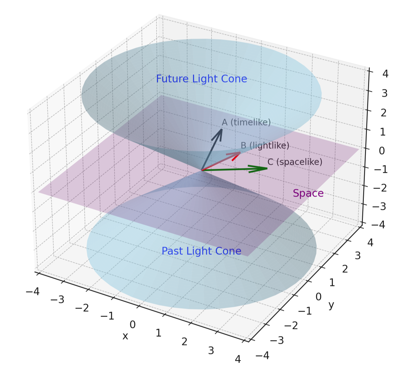
• Timelike: $s^2>0$. There exists a frame in which the events occur at the same spatial point but different times; a slower-than-light traveler can go from A to B.
• Lightlike (null): $s^2=0$. Only a light signal can connect them.
• Spacelike: $s^2<0$. There exists a frame in which the events are simultaneous but different places; no signal can connect them without exceeding $c$.

At any event the set $ds^2=0$ forms the light cone with generators $x=\pm ct$ (in $1+1$ dimensions). The interior is timelike, the exterior spacelike. Lorentz transformations preserve this cone, so all inertial observers agree on causal possibilities even if they disagree on times and distances.

5.3.3 Proper time and worldlines

A worldline is a curve $x^\mu(\lambda)$ describing an object’s history. For timelike motion the clock carried by the object ticks the proper time

Integrating gives the elapsed time on that clock:

Among all timelike curves connecting the same endpoints in flat spacetime, inertial motion maximizes $\Delta\tau$. This geometric statement resolves the twin scenario: the traveling twin takes a non-inertial path with smaller proper time.

5.3.4 Four-velocity and four-acceleration

Define the four-velocity

Using $ds^2=c^2 d\tau^2$ one finds the normalization

Writing spatial velocity $\mathbf v=d\mathbf x/dt$ and $\gamma=1/\sqrt{1-v^2/c^2}$ gives

The four-acceleration $a^\mu = du^\mu/d\tau$ satisfies an orthogonality identity

meaning acceleration is purely “spacelike” in the instantaneous rest frame. These tools streamline relativistic dynamics (§5.5).

5.3.5 Lorentz transformations as hyperbolic rotations

A boost along $x$ with speed $v$ can be written using $\beta=v/c$ and $\gamma=1/\sqrt{1-\beta^2}$:

The matrix $\Lambda^\mu{}_\nu$ of this transformation obeys the invariance condition

This is analogous to how ordinary rotations preserve Euclidean lengths. Indeed, if we define the rapidity $\eta$ by $\beta=\tanh\eta$, then

and the boost becomes a hyperbolic rotation in the $ct$–$x$ plane. Composition of collinear boosts simply adds rapidities. That is why velocity composition has the non-linear Einstein form yet remains associative in rapidity space.

5.3.6 Reading Minkowski diagrams

A Minkowski diagram displays $ct$ vertically and $x$ horizontally. Light rays draw lines at slopes $\pm 45^\circ$ (since $x=\pm ct$ in units with $c=1$). Some practical rules:

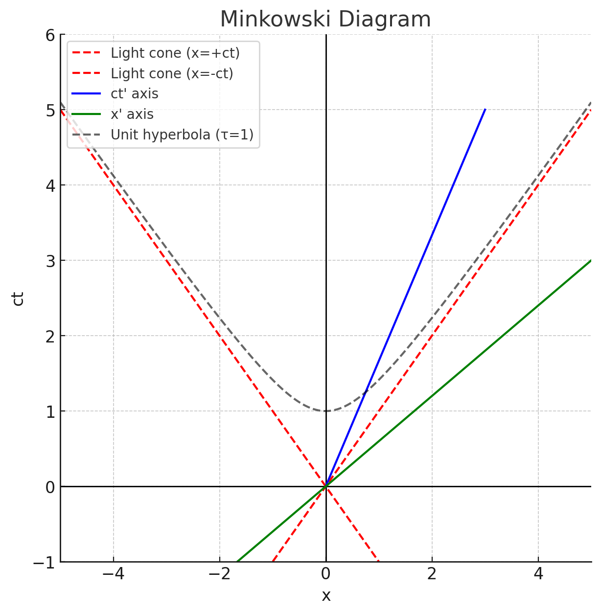
1. Axes of a moving frame. The $x'$ axis is the line of events with $t'=0$, which tilts upward; the $ct'$ axis is the worldline $x'=0$, which tilts right. The two axes are symmetric with respect to the light cone.
2. Simultaneity slices. Lines of constant $t'$ are not horizontal unless $v=0$; that is the relativity of simultaneity made visible.
3. Unit calibration. The unit hyperbola $ct=\sqrt{x^2+c^2\tau^2}$ encodes proper time ticks; Loedel diagrams use symmetric scaling to keep both frames drawn with the same light-cone angle.
4. Causality test. If an event B lies outside A’s light cone, no worldline with $|v|<c$ connects A to B. Event order for spacelike pairs can flip under boosts; for timelike pairs it cannot.

Diagrams are not just pictures; they are calculators for ordering, time dilation, length contraction, and simultaneity shift.

5.3.7 Causality, no-signaling, and why $c$ is a speed limit

Suppose there existed a signal with speed $u>c$ in some frame. A boost can be found that flips the temporal order of emission and reception for a spacelike separation. Combined with “you can send signals both ways,” this makes a closed causal loop—a paradox. Special relativity avoids this by forbidding superluminal signaling: physical worldlines are timelike or null, never spacelike. As a corollary, there are no perfectly rigid bodies; attempts to jerk one end of a rod cannot simultaneously affect the other end because stress information travels at material sound speeds $<c$.

Microcausality in field theory is the quantum echo of this rule: field operators at spacelike separations commute so that measurements cannot influence one another.

5.3.8 Energy–momentum as a four-vector (preview)

Later we will use the energy–momentum four-vector

with invariant

This single relation encodes both the rest-energy $E_0=mc^2$ and the dispersion $E^2=(pc)^2+(mc^2)^2$. The conservation of $p^\mu$ across interactions is a compact, frame-independent way to do dynamics.

5.3.9 Accelerated motion in flat spacetime

Even without gravity we can treat accelerated observers. A worldline with constant proper acceleration $a$ in the $x$ direction traces a hyperbola,

which stays asymptotic to the light lines $x=\pm ct$. Proper acceleration is what an accelerometer reads; it is invariant, unlike coordinate acceleration which depends on frame.

Accelerated frames bring in Rindler coordinates and horizons even in flat spacetime—useful stepping stones toward the equivalence principle (§5.8).

5.3.10 Tensors and index gymnastics (minimal toolkit)

A four-vector transforms as $A'^\mu=\Lambda^\mu{}_\nu A^\nu$. Lowering and raising indices uses $\eta_{\mu\nu}$ and its inverse:

Lorentz-invariant scalars are built by contracting indices, for example $A_\mu B^\mu$. The electromagnetic field appears as an antisymmetric tensor $F_{\mu\nu}$; writing Maxwell’s equations in this language exposes symmetry and automatically preserves causality, because $F_{\mu\nu}$ transformations keep light cones intact.

5.3.11 What changes, what stays the same

• Changes: time intervals, lengths, and simultaneity slices between frames.
• Stays the same: the light cone, the interval $ds^2$, proper time $\tau$, and causal order for timelike-related events.

This is the mantra of relativistic reasoning: compute invariants first; everything else is perspective.

5.3.12 Quick problem templates

1. Is A able to influence B? Compute $s^2$. If $s^2<0$, no. If $s^2=0$, only with light. If $s^2>0$, yes with subluminal motion.
2. How old is the traveler? Integrate $d\tau=\sqrt{1-v^2/c^2}\,dt$ along the actual velocity profile.
3. What does a moving observer see? Apply the boost; redraw axes; use the simultaneity formula and length contraction as needed.

In summary: Minkowski spacetime packages relativity into geometry. The metric $ds^2=c^2dt^2-d\mathbf x^2$ defines light cones and proper time; boosts are hyperbolic rotations preserving those cones. Causality becomes a geometric constraint—worldlines must stay inside or on light cones—and dynamics a story of four-vectors that transform covariantly. Once you think in intervals, cones, and rapidities, the paradoxes evaporate and the calculations streamline.

5.4 Relativistic Dynamics

Kinematics told us how coordinates transform. Dynamics asks how momentum, energy, and forces behave so that the laws look the same to every inertial observer. The guiding idea is simple: build everything from Lorentz-invariant or covariant objects so that physical predictions do not depend on the frame.

5.4.1 Four-momentum and the energy–momentum relation

Define the four-velocity and four-momentum

with $d\tau$ the proper time. Using $u^\mu u_\mu = c^2$, we have

The temporal component defines energy

and spatial part defines momentum

The invariant magnitude of $p^\mu$ gives the master relation

or, written in scalars,

This reduces at low speeds to familiar Newtonian forms. Expanding $\gamma$ for $v \ll c$,

so the Newtonian kinetic energy appears as the first correction above the rest energy $m c^2$.

5.4.2 Work, power, and the relativistic force law

Keep the Newtonian definitions but use relativistic $\boldsymbol p$ and $E$:

With $\boldsymbol p=\gamma m \boldsymbol v$ one finds

Decomposing into parts parallel and perpendicular to $\mathbf v$ gives the compact rules

So as speeds approach $c$, the same applied force yields smaller acceleration, especially along the direction of motion. The speed limit is thus dynamical as well as kinematical.

It is often cleaner to package force into a four-vector. Define the four-force

which automatically satisfies an orthogonality identity

because $p^\mu p_\mu$ is constant. In §5.6 we will specialize this to charged particles in electromagnetic fields.

5.4.3 Action principle and the free-particle Lagrangian

Relativistic dynamics drops out of a geometric action. For a neutral particle,

In a given frame, $ds = c\,dt\,\sqrt{1 - v^2/c^2}$, so the Lagrangian is

The canonical momentum and Hamiltonian follow:

Thus the energy–momentum relations are not assumptions but consequences of the variational principle built from the invariant length of worldlines.

When a particle carries charge $q$ and interacts with an electromagnetic four-potential $A_\mu=(\phi/c,\,-\boldsymbol A)$, the minimal-coupling action adds $q\int A_\mu dx^\mu$. In ordinary variables the Lagrangian becomes

whose Euler–Lagrange equations yield the Lorentz force in covariant form (shown in §5.6).

5.4.4 Momentum and energy balance in collisions

Because four-momentum is conserved,

This single vector equation encodes both ordinary momentum conservation and energy conservation in all frames. Squaring both sides produces frame-invariant relations useful for particle reactions.

A key invariant is the Mandelstam $s$ for two particles with four-momenta $p_1,p_2$:

In the center-of-momentum (CM) frame, $s = (E_{\text{CM}}/c)^2$, so $E_{\text{CM}} = \sqrt{s}\,c$. In a lab frame where target $b$ is at rest and beam $a$ has energy $E_a$,

or, more transparently,

At threshold for producing final particles of total rest mass $M_{\text{final}}$, the CM kinetic energy just vanishes, so

and the required lab energy of the beam is

As a concrete example, consider $p + p \to p + p + \pi^0$ with one proton at rest. Taking $m_p$ and $m_\pi$ as the rest masses, $M_{\text{final}} = 2 m_p + m_\pi$, and the formula above gives the familiar multi-GeV threshold for pion production in fixed-target experiments.

5.4.5 Center-of-momentum frame and invariant mass of a system

For any isolated system, define the total four-momentum

The invariant

is the system’s invariant mass. In the CM frame $\boldsymbol P=\boldsymbol 0$, so $M_{\text{sys}} c^2 = E_{\text{CM}}$. Crucially, $M_{\text{sys}}$ is not just the sum of rest masses; it includes kinetic and binding energies. For example, a box containing radiation has larger $M_{\text{sys}}$ than the empty box, because photons carry energy and momentum even though their individual rest masses are zero.

5.4.6 Massless particles and dispersion

For $m=0$ the invariant relation becomes

The four-velocity is undefined for lightlike worldlines, but the four-momentum remains finite and transforms correctly. A photon’s energy relates to frequency by $E=h\nu$, consistent with $p=h/\lambda$ and Maxwell’s waves moving at $c$. Massive particles cannot reach $c$ because that would require $\gamma \to \infty$, hence infinite energy.

5.4.7 Dynamics with constraints and radiation reaction (glimpse)

For charged particles, the Lorentz force law reads in three-vector form (derived covariantly in §5.6)

Because accelerating charges radiate, an additional radiation reaction force arises at higher fidelity. Its classical expression (Abraham–Lorentz–Dirac) is subtle and can lead to runaways; in practice one uses approximations consistent with the external fields. The key point for dynamics: energy lost to radiation must be accounted for in $dE/dt$.

5.4.8 Proper acceleration and hyperbolic motion

A trajectory with constant proper acceleration $a$ along $x$ satisfies

Differentiation gives speed

So even with constant proper acceleration, the coordinate acceleration decreases as $v$ approaches $c$, asymptotically respecting the speed limit while proper time accumulates at a slower rate.

5.4.9 Quick toolbox for problems

• Use $p^\mu=(E/c,\,\boldsymbol p)$ and conserve four-momentum; square once if you want frame-free answers.
• For rockets or beams, compute power with $dE/dt=\boldsymbol F\cdot\boldsymbol v$ and relate thrust to $d\boldsymbol p/dt$.
• Choose the CM frame to minimize algebra; transform back with the Lorentz formulas of §5.3.
• Remember $M_{\text{sys}}$ includes kinetic and binding energy; “mass of a system” is an invariant, not just the sum of constituent rest masses.

In summary: Relativistic dynamics packages energy and momentum into a single four-vector that obeys $E^2=(pc)^2+(mc^2)^2$. Forces change momentum via $d\boldsymbol p/dt$ and do work at rate $\mathbf F\cdot\mathbf v$, while the covariant four-force $K^\mu=dp^\mu/d\tau$ keeps orthogonality to $u^\mu$. Collisions are clean in terms of invariants like $s$ and the system mass $M_{\text{sys}}$. All of it is geometry: conserve four-vectors and respect the light cone, and dynamics becomes as straightforward as kinematics.

5.5 Electromagnetism in Relativistic Form

Maxwell’s theory already smells relativistic. Here we make that symmetry explicit: package $\boldsymbol E$ and $\boldsymbol B$ into a single field tensor, write the equations and forces in four-dimensional form, and expose the invariants that every observer agrees on.

5.5.1 Four-current, four-potential, and the field tensor

Combine charge density and current into the four-current

Combine scalar and vector potentials into the four-potential

Define the antisymmetric electromagnetic field tensor

With metric $\eta_{\mu\nu}=\mathrm{diag}(1,-1,-1,-1)$ (SI units),

So $\boldsymbol E$ and $\boldsymbol B$ are not separate things; they are different facets of the same tensor.

5.5.2 Maxwell’s equations as two short tensor laws

All four Maxwell equations compress to just two:

Using the dual tensor $\tilde F^{\mu\nu} \equiv \tfrac12 \epsilon^{\mu\nu\alpha\beta} F_{\alpha\beta}$, the second line becomes

Written this way, Lorentz covariance is manifest: the equations keep the same form in every inertial frame.

5.5.3 Lorentz force in one line

A particle of charge $q$ and four-velocity $u^\mu$ obeys

Splitting into time and space parts gives the familiar three-vector form

One covariant equation, every frame happy.

5.5.4 Gauge symmetry and wave equations

Gauge transformations leave physics unchanged:

In the Lorenz gauge

Maxwell’s equations reduce to wave equations for the potential:

where $\square \equiv \partial_\mu\partial^\mu = \frac{1}{c^2}\frac{\partial^2}{\partial t^2}-\nabla^2$ is the d’Alembertian.

5.5.5 How fields transform: boosts mix $\,\boldsymbol E$ and $\,\boldsymbol B$

Relativity treats “electric” and “magnetic” as frame-dependent decompositions of one tensor. For a boost with velocity $\boldsymbol v$,

For a boost along $x$ with speed $v$,

A pure electric field in one frame generally appears as a mix of electric and magnetic fields in another.

5.5.6 Two Lorentz invariants (frame-proof diagnostics)

Two independent Lorentz scalars diagnose the field:

In SI variables,

For a plane wave,

so $\mathcal I_1=\mathcal I_2=0$ (a null field). If $\mathcal I_1<0$ and $\mathcal I_2=0$, there exists a frame where the field is purely electric; if $\mathcal I_1>0$ and $\mathcal I_2=0$, a purely magnetic frame exists.

5.5.7 Field energy–momentum and stresses

Package energy, momentum, and stresses into the electromagnetic stress–energy tensor

Its (non)conservation in the presence of sources reads

Components:

So $T^{00}$ is energy density, and $T^{0i}$ encodes momentum density via the Poynting vector $\boldsymbol S$. The spatial block $T^{ij}$ (Maxwell stress tensor) gives pressures and tensions exerted by fields.

5.5.8 Lagrangian density (one line to rule them all)

The field-theory origin story fits on one line:

Varying $A_\mu$ yields Maxwell’s equations; gauge symmetry leads, via Noether’s theorem, to charge conservation $\partial_\mu J^\mu=0$.

5.5.9 Fields of moving charges (why magnetism appears)

Boost a static Coulomb field and you get an anisotropically compressed electric field plus a magnetic field. In other words,

Magnetism is not a separate force; it is the frame-dependent slice of $F_{\mu\nu}$.

5.5.10 Quick recap

• The field is $F_{\mu\nu}$, the sources are $J^\mu$, and the potential is $A^\mu$
• Maxwell’s equations: $\partial_\mu F^{\mu\nu}=\mu_0 J^\nu$ and $\partial_\mu \tilde F^{\mu\nu}=0$
• Lorentz force: $dp^\mu/d\tau = q F^\mu{}_{\ \nu} u^\nu$
• Boosts mix $\boldsymbol E$ and $\boldsymbol B$, but the invariants $\mathcal I_1,\mathcal I_2$ stay fixed
• Energy–momentum flows with $T^{\mu\nu}$; $\boldsymbol S=(1/\mu_0)\boldsymbol E\times\boldsymbol B$

In summary: Electromagnetism is not two fields but one tensor $F_{\mu\nu}$. Lorentz transformations change how $\boldsymbol E$ and $\boldsymbol B$ look, not what the physics is. Writing everything in four-dimensional form makes covariance obvious, sharpens what’s invariant, and turns long vector calculus into compact geometry.

5.6 Relativistic Optics and Technology

Special relativity reshapes how light looks when sources or observers move fast. The result is a small toolkit—Doppler, aberration, and beaming—that explains phenomena from quasar jets to accelerator light and enables technologies from GPS to synchrotron X-ray sources. This section packages the main formulas, shows what is invariant, and sketches applications.

5.6.1 Relativistic Doppler: frequency shift as kinematics

For motion strictly along the line of sight with speed $v$ (define $\beta \equiv v/c$), the observed frequency is related to the emitted one by the Doppler factor

Approaching sources are blueshifted, receding are redshifted:

At small speeds this reduces to the classical shift. For purely transverse relative motion (source moves sideways), there is still a redshift due to time dilation alone:

5.6.2 Aberration of light: where the rays appear to come from

Motion squeezes apparent angles toward the direction of travel. If a light ray makes angle $\theta$ with the $x$-axis in $S$ and $\theta'$ in $S'$ that moves at speed $v$ along $+x$, then

Equivalently,

Starlight appears displaced (aberration), and radiation patterns are forward-beamed at high $\gamma$.

5.6.3 Beaming and intensity transformation

Specific intensity satisfies a powerful invariant:

Hence for a boost with Doppler factor $\mathcal D$,

Integrating over frequency (bolometric intensity) gives

This headlight effect makes relativistic jets look dramatically brighter when pointed near our line of sight and dimmer when pointed away. Photons are not created; phase-space density is simply redistributed by the boost.

5.6.4 Synchrotron and curvature radiation

Charged particles forced into curved paths radiate. In circular motion of radius $\rho$ at ultra-relativistic speed, the spectrum peaks near the critical frequency

The total radiated power for motion with curvature $\rho$ scales strongly with $\gamma$,

(up to the standard SI prefactor). Two key consequences: (i) high-energy electrons in magnetic fields produce broad-band synchrotron radiation (radio to X-ray), and (ii) storage rings and undulators become bright, tunable light sources (synchrotron facilities, FELs) used for protein crystallography, materials science, and nanolithography.

5.6.5 Brightness temperatures and spectra (quick rules)

For a power-law emitter with $I'_{\nu'}\propto \nu'^{\,\alpha}$, the observed spectrum under a boost obeys

Isotropic rest-frame emission becomes anisotropic: apparent opening angles scale like $\sim 1/\gamma$, and variability timescales shrink by $1/\mathcal D$ (time compression). These scalings underlie inferences of bulk Lorentz factors in blazars and gamma-ray bursts.

5.6.6 Radar and lidar at speed: closing speed is not “just add”

When platforms move relativistically, measured beat frequencies in radar/lidar follow the same Doppler algebra. For monostatic radar with target closing speed $v$ along the line of sight, the round-trip shift accumulates twice:

In the low-$v$ limit this reduces to the familiar $2v/c$ formula. At high $v$, use the exact $\mathcal D$ to avoid systematic bias.

5.6.7 GPS and clocks: engineering with relativity

Modern navigation is a timing game. In special relativity, a clock moving at speed $v$ ticks slower by $\gamma$:

Satellite clocks thus run slow due to orbital speed (special relativity) but fast due to higher gravitational potential (general relativity, §5.8). Flight software pre-biases clock frequencies and continuously corrects time using relativistic models; without these, position errors would grow to kilometers per day.

5.6.8 Imaging at relativistic speeds (thought experiments to lab)

If a camera moves near $c$ past a scene, aberration funnels most photons into a forward cone; Doppler shifts move spectra; and Terrell rotation (a geometry effect) makes objects appear rotated rather than squashed. Lab analogs show pieces of this: relativistic electron bunches “see” laser pulses Doppler-upshifted into X-rays (inverse Compton sources), enabling compact X-ray generation.

5.6.9 Cherenkov versus Doppler (don’t mix them)

Cherenkov radiation occurs when a charge moves through a medium faster than light’s phase speed in that medium. It is not superluminal in vacuum and does not violate relativity. In contrast, relativistic Doppler and aberration are vacuum kinematics. Both appear in detectors and astrophysics, but they answer different questions.

5.6.10 Practical crib sheet

• Doppler factor: $\displaystyle \mathcal D=\sqrt{\frac{1+\beta}{1-\beta}}$; use $\nu_{\text{obs}}=\mathcal D\,\nu_{\text{emit}}$
• Transverse Doppler: $\displaystyle \nu_{\text{obs}}=\nu_{\text{emit}}/\gamma$
• Aberration: $\displaystyle \cos\theta'=\frac{\cos\theta-\beta}{1-\beta\cos\theta}$
• Intensity: $I_\nu/\nu^{3}$ invariant $\Rightarrow\ I_\nu=\mathcal D^{3} I'_{\nu'}$; bolometric $I=\mathcal D^{4} I'$
• Synchrotron: $\displaystyle \omega_c=(3/2)\gamma^{3} c/\rho$; power $\propto \gamma^{4}/\rho^{2}$

In summary: Relativistic kinematics tilts light cones into everyday engineering. Doppler and aberration set what frequencies we detect and where sources appear; beaming and intensity invariants set how bright they look; synchrotron formulas govern radiation from bent charges. The same few relations explain cosmic jets, power ultra-bright light sources, and keep your phone’s map honest.

5.7 Equivalence Principle: Toward General Relativity

Special relativity rebuilt kinematics as geometry. Gravity finishes the renovation by changing the geometry itself. The doorway is Einstein’s equivalence principle: locally, a uniform gravitational field is indistinguishable from a uniformly accelerated frame. From this one idea flow gravitational redshift, the universality of free fall, and ultimately the field equations of general relativity.

5.7.1 Inertial vs gravitational mass: the clue

In Newtonian mechanics you meet two masses: inertial $m_{\mathrm i}$ (resistance to acceleration) and gravitational $m_{\mathrm g}$ (how strongly gravity pulls). Experiments show they are equal to astonishing precision, so motion in a gravitational field is independent of composition. This universality of free fall hints that gravity is not a force in the usual sense but a property of spacetime affecting all matter the same way.

Einstein took the equality $m_{\mathrm g}=m_{\mathrm i}$ as a postulate and asked: what worldview makes this identity natural?

5.7.2 Einstein’s elevator: redshift and light bending—without gravity

Imagine a small laboratory (an elevator) in deep space, initially at rest. Now fire its rockets so it accelerates upward with constant acceleration $a$. A laser at the floor emits upward; by the time the light reaches the ceiling, the ceiling has picked up speed and sees a Doppler redshift. Over a height $h$, the fractional shift is

Replace $a$ by $g$ and you have the gravitational redshift in a uniform field:

Same lab, different stunt: toss a horizontal light pulse across the cabin. During the flight time $t\approx \ell/c$, the cabin accelerates downward relative to the beam, so the light appears to curve. By equivalence, light should also bend near a mass. The elevator thought experiment already whispers the core GR predictions.

5.7.3 Local inertial frames: gravity can be transformed away (but only locally)

At any spacetime event you can choose coordinates that make physics look like special relativity to first order. Technically: at a point $P$ there exist local inertial coordinates with

In such a frame, freely falling test bodies move on straight lines through $P$ and clocks behave as in SR—locally. You cannot make gravity vanish everywhere because second derivatives of the metric (curvature) remain. Those second derivatives encode tidal effects.

5.7.4 Geodesics: free fall as straightest possible paths

In GR, free fall is not “force-driven” motion; it is geodesic motion—extremal proper time curves in a curved manifold. The equation of motion is

Here $\Gamma^{\mu}{}_{\alpha\beta}$ are the Christoffel symbols built from $g_{\mu\nu}$. In flat spacetime they can be set to zero globally; in curved spacetime they vanish only at a point by going to a local inertial frame.

5.7.5 Curvature and tides: geodesic deviation

Two nearby freely falling particles with separation $\xi^\mu$ and 4-velocity $u^\mu$ obey the geodesic deviation equation

$R^{\mu}{}_{\nu\alpha\beta}$ is the Riemann curvature tensor. If $R=0$, freely falling worldlines remain parallel (no tides). Nonzero curvature makes them focus or defocus—that is gravity in GR. The “gravitational field” is not a vector; it is geometry.

5.7.6 From equivalence to field equations

Einstein asked for the simplest field equations that

1. reduce to Newtonian gravity when fields are weak and speeds are slow,
2. conserve energy–momentum, and
3. are generally covariant (valid in any coordinates).

The answer is the Einstein field equation

Optionally one may add a cosmological constant $\Lambda$ on the left $(+\Lambda g_{\mu\nu})$; we omit it below for simplicity. $T_{\mu\nu}$ is the stress–energy tensor of matter and fields. Geometry $G_{\mu\nu}$ on the left, sources $T_{\mu\nu}$ on the right—the slogan is “matter tells spacetime how to curve; spacetime tells matter how to move.”

5.7.7 Newtonian limit: recovering Poisson’s law

Consider a static, weak field so that the metric component is

where $\Phi$ is the Newtonian potential with $|\Phi|/c^{2}\ll 1$. Insert this ansatz into the field equations and keep lowest order in $1/c^{2}$. One obtains

and free-fall trajectories reduce to $\boldsymbol a = -\nabla\Phi$. GR passes the sanity check: it contains Newton as the slow-motion, weak-field limit.

5.7.8 Gravitational time dilation and redshift (proper time in a static field)

For a stationary metric, a clock at fixed spatial coordinates ticks proper time

Near Earth, with $g_{00}\approx 1+2\Phi/c^{2}$ and small potential differences $\Delta\Phi\approx g\,\Delta h$, the fractional rate shift between altitudes is

This is why GPS satellite clocks (higher $\Phi$) run faster than identical ground clocks and must be pre-biased and corrected.

5.7.9 Accelerated frames and Rindler coordinates (flat spacetime warm-up)

Uniformly accelerated observers in flat spacetime cover a Rindler wedge. One convenient chart in $1+1$ dimensions uses parameters $(\rho,\eta)$ related to inertial $(ct,x)$ by

In these coordinates the metric reads

Clocks at different $\rho$ tick at different rates, mimicking gravitational redshift. Equivalence tells us that many “accelerated frame” effects have gravitational analogs when curvature is small over the lab.

5.7.10 Light deflection, delay, and perihelion (previews)

Full GR predicts quantitative effects that can be phrased through the metric. For a light ray grazing a mass $M$ with impact parameter $b$, the bending angle is

Signals skimming a mass experience an extra Shapiro time delay tied to $g_{00}$ and spatial curvature. Bound orbits in curved spacetime precess; Mercury’s perihelion shift (after subtracting planetary perturbations) matches GR. We will collect classic tests in §5.9.

5.7.11 What the equivalence principle really asserts

• Weak equivalence (universality of free fall): test bodies with negligible self-gravity follow the same trajectories given identical initial conditions in a given gravitational field
• Einstein equivalence: in any local freely falling frame, non-gravitational physics reduces to special relativity; outcomes are independent of where and when the experiment is performed

Equivalence does not say gravity can be transformed away everywhere, nor that “gravity is a fictitious force.” It says that locally you can remove gravitational effects by free fall, leaving only curvature (tidal terms) as the invariant content.

5.7.12 Minimal problem kit

• From a given metric $g_{\mu\nu}$, compute $d\tau=\sqrt{g_{00}}\,dt$ for clocks at rest and compare rates
• For slow motion in a weak field, read off $\Phi$ from $g_{00}\approx 1+2\Phi/c^{2}$ and recover Newtonian limits
• To track free fall, set up the geodesic equation with $\Gamma^{\mu}{}_{\alpha\beta}(g)$ and integrate, or use conserved quantities from symmetries (Killing vectors)

In summary: The equivalence principle recasts gravity as geometry. Locally you can fall away the field, but you cannot eliminate curvature—tidal effects are the real, frame-invariant residue. Demanding a theory that honors equivalence, conserves energy–momentum, and recovers Newton leads to Einstein’s equation $G_{\mu\nu}=(8\pi G/c^{4})T_{\mu\nu}$. From redshift to light bending to clock rates in orbit, the elevator thought experiment graduates into a full-blown theory of curved spacetime.

5.8 Tests and Frontiers

Relativity is not a vibe check; it is an experiment magnet. From Mercury’s orbit to gravitational waves and black-hole images, the theory keeps passing increasingly savage tests. This section hits the classics, then pushes to frontiers where precision, strong gravity, or cosmic scales stress the model.

5.8.1 Classic tests in the weak field

Perihelion advance of Mercury. Newtonian gravity plus planetary perturbations misses a small excess. For a bound orbit with semi-major axis $a$ and eccentricity $e$ around mass $M$, GR predicts per orbit

Deflection of light. A light ray grazing a mass $M$ with impact parameter $b$ is bent by

This doubles the naive Newtonian-particle estimate because spacetime curvature bends both time and space.

Gravitational redshift. In a static weak field, clocks at higher potential tick faster. For small height difference $h$ near Earth with acceleration $g$,

Shapiro time delay. Radar signals skimming a massive body arrive late compared with Euclidean expectations. For a round trip past mass $M$ with appropriate geometry,

The logarithm is the telltale GR signature.

5.8.2 Equivalence principle tests

If all uncharged test bodies fall the same way, the Eötvös parameter must be tiny

Modern torsion balances, atom interferometers, and lunar laser ranging constrain $\eta$ to be extremely small, keeping Einstein’s elevator happily indistinguishable from a lab in free fall.

5.8.3 Binary pulsars and gravitational radiation

A compact binary loses orbital energy to gravitational waves, shrinking its period. In GR the period derivative depends on the chirp mass $M_{c}$

For a quasi-circular binary with orbital period $P$,

Radio timing of pulsars matches this prediction and measures $M_{c}$ cleanly. Strong-field, radiative GR survives the check.

5.8.4 Direct gravitational waves and chirps

Interferometers measure a dimensionless strain $h=\Delta L/L$ from passing ripples. For a quasi-circular inspiral, the gravitational-wave frequency $f$ accelerates according to

From $f(t)$ one extracts $M_{c}$ and distances without a cosmic distance ladder. Multi-detector triangulation localizes sources; polarization and phasing test GR’s waveform templates.