3 Thermodynamics

3.1 Introduction: Heat and the Quest for Order

In the eighteenth and nineteenth centuries, the enigma of heat dominated both practical engineering and philosophical speculation. Was heat a fluid that flowed invisibly from hot to cold bodies, a substance called caloric? Or was it simply the ceaseless motion of particles too small to perceive? The answer to this question mattered not only for academic pride but also for the future of industry and empire. Heat drove the engines of the Industrial Revolution, and to master it was to master power itself.

The Caloric Hypothesis

The caloric theory described heat as an indestructible, weightless fluid that could neither be created nor destroyed, only transferred. To many, this seemed reasonable: when one object became hot, another cooled, as though some hidden substance had flowed. The caloric theory allowed scientists to calculate flows and capacities, and it provided a sense of conservation. Yet cracks in the theory appeared whenever experiment pressed too hard.

The most dramatic blow came from Benjamin Thompson, Count Rumford, an American-born adventurer who defected to the British side during the American Revolution and later became a Bavarian court scientist. In the 1790s, while supervising the boring of cannons at a Munich arsenal, Rumford noticed that seemingly endless amounts of heat could be generated by friction. He argued that if caloric were a conserved fluid, the supply within a cannon would quickly run dry. Instead, boring produced heat without limit. Rumford concluded that heat was not a substance at all but rather motion—a view ahead of its time, and one that foreshadowed the kinetic theory of gases.

Industry and Engines

Meanwhile, the Industrial Revolution turned questions of heat from metaphysics into economics. Factories devoured coal, and steam engines pumped mines dry and propelled trains across continents. Nations competed to harness heat with greater efficiency. James Watt’s improvements to the steam engine had already changed the landscape of industry, but fundamental questions remained unanswered: Was there a theoretical ceiling on engine efficiency? Could heat be entirely converted into work? These were no longer idle musings; they were matters of survival in a rapidly mechanizing world.

Into this atmosphere was born Sadi Carnot (1796–1832), the son of Lazare Carnot, a general and statesman of Revolutionary France. Though trained as a military engineer, Sadi possessed the spirit of a theorist. In 1824, at only 27 years old, he published Réflexions sur la puissance motrice du feu (Reflections on the Motive Power of Fire). His work asked a deceptively simple but revolutionary question: What is the maximum efficiency any heat engine can achieve, regardless of design? Carnot’s answer did not rely on molecules—he still spoke in the language of caloric—but his logic was so profound that it outlived the very paradigm he employed. His reasoning gave birth to the concept of reversible processes and planted the seeds of entropy, though the term itself had not yet been coined.

From Carnot to Clausius and Kelvin

Carnot’s work might have been forgotten had it not been for later reformulations. Rudolf Clausius (1822–1888) took Carnot’s reasoning and recast it in terms of energy and heat as forms of motion. In doing so, he coined the term entropy and declared the now-famous principle: “The entropy of the universe tends toward a maximum.” Clausius gave thermodynamics its irreversible character, identifying a law that no process in the universe can escape.

At nearly the same time, William Thomson, Lord Kelvin (1824–1907), expanded Carnot’s ideas into a universal principle. He introduced the absolute temperature scale, eliminating arbitrary references and grounding thermodynamics in a universal metric. It was Kelvin who popularized the distinction between reversible and irreversible processes and who warned that one day the universe might experience a “heat death,” a state of uniform temperature where no free energy remains to do work.

The Broad Reach of Thermodynamics

Thermodynamics was never only about engines. James Clerk Maxwell introduced his famous thought experiment of the “demon” that could seemingly violate the second law by sorting molecules. This playful idea sparked debates that extended into the twentieth century and eventually birthed the thermodynamics of information. Ludwig Boltzmann, perhaps the most tragic and brilliant figure of the discipline, supplied the statistical underpinnings: entropy, he argued, is proportional to the logarithm of the number of microscopic configurations compatible with a macroscopic state. His equation,

was so fundamental that it was carved on his tombstone in Vienna.

The story of thermodynamics is thus not merely one of physics but of philosophy. It explains why no engine can be perfect, why time flows irreversibly, why life consumes energy to maintain order, and why the universe itself may one day fade into equilibrium. Few scientific disciplines have such universal reach: from the friction of Rumford’s cannons to the evaporation of black holes, the same principles rule.

Toward the Laws of Thermodynamics

From these investigations emerged the celebrated laws of thermodynamics:

1. Zeroth Law: If two systems are each in thermal equilibrium with a third, they are in equilibrium with each other—justifying the concept of temperature.
2. First Law: Energy cannot be created or destroyed, only transformed.
3. Second Law: Entropy of an isolated system never decreases; natural processes are irreversible.
4. Third Law: As temperature approaches absolute zero, entropy approaches a constant minimum.

Together, these laws form a framework more universal than Newton’s mechanics, for they apply not only to masses and forces but to any system—chemical, biological, or even cosmological.

In summary: The quest to understand heat was born from industry, shaped by daring experiments, and elevated by profound theoretical insight. From caloric to entropy, from steam engines to the universe, thermodynamics teaches us that energy is conserved, entropy grows, and order must be purchased at a cost. It is both a practical science and a philosophical compass, pointing always toward the limits of what is possible in nature.

3.2 Carnot and the Ideal Engine

The history of thermodynamics pivots on a young French engineer named Nicolas Léonard Sadi Carnot (1796–1832). Born into a family steeped in the politics and science of Revolutionary France, Sadi inherited both an engineer’s rigor and a philosopher’s curiosity. His father, Lazare Carnot, had been called the “Organizer of Victory” for his role in the Revolutionary Wars, a strategist who combined mathematics with military art. Sadi, however, was destined to fight a different battle: the war to understand heat.

A Life Brief but Profound

Carnot’s life was tragically short—he died of cholera at 36—but in those years he produced a single book that altered science forever: Réflexions sur la puissance motrice du feu (Reflections on the Motive Power of Fire, 1824). At that time, France’s industrial future depended on steam engines. Britain led the revolution with James Watt’s designs, and French engineers wondered: could their machines ever match or surpass the English? Carnot took this practical concern and elevated it to a fundamental question:

What is the maximum efficiency of any engine operating between two heat reservoirs?

It was a breathtakingly abstract question for its time. Carnot did not know the atomic theory of matter, nor the kinetic view of heat as molecular motion. He still wrote in the language of caloric—the hypothetical fluid of heat. Yet by sheer logical reasoning, Carnot anticipated the essential truth: efficiency is limited by temperature alone.

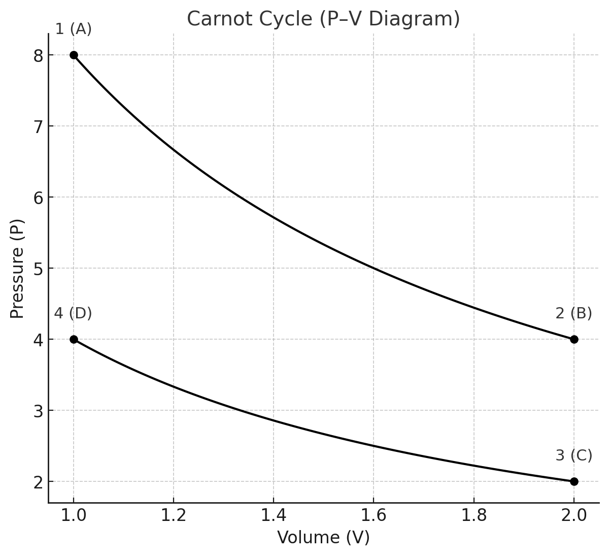
The Carnot Cycle

Carnot imagined an idealized engine performing a cycle composed of four reversible processes:

1. Isothermal expansion at (T_h).
   The working substance (say, an ideal gas) is placed in contact with a hot reservoir at temperature (T_h). It expands while absorbing heat (Q_h). Because the process is isothermal, the internal energy (U) of the gas remains constant; all heat absorbed is converted into work.

   $$Q_h = W_{\text{exp}} = nRT_h \ln\!\left(\frac{V_b}{V_a}\right).$$

2. Adiabatic expansion.
   The system is thermally isolated. It continues to expand, doing work on the surroundings, but now cooling from (T_h) to (T_c). No heat flows: (\delta Q = 0). For an ideal gas, this follows the relation:

   $$T V^{\gamma-1} = \text{constant}, \qquad PV^\gamma = \text{constant}.$$

3. Isothermal compression at (T_c).
   The system is placed in contact with the cold reservoir. The surroundings compress the gas, and the gas rejects heat (Q_c) to the reservoir. Internal energy again remains constant.

   $$Q_c = nRT_c \ln\!\left(\frac{V_d}{V_c}\right).$$

4. Adiabatic compression.
   Finally, the system is isolated again. Compression raises its temperature from (T_c) back to (T_h), restoring the initial state.

At the end of the cycle, the system has returned to its starting point. By definition of a cycle, internal energy change is zero ((\Delta U = 0)). Therefore the work performed by the system equals the net heat absorbed:

The efficiency is thus

Efficiency Depends Only on Temperature

For a reversible isothermal process, the entropy exchanged is

Because the cycle is closed and reversible, the total entropy change is zero:

Therefore,

This is the Carnot efficiency—the absolute upper bound for any heat engine operating between two temperatures. The remarkable fact is that it depends only on (T_h) and (T_c), not on the working substance or the details of the engine. Steam, air, helium, or even a hypothetical perfect fluid—all obey the same constraint.

Implications of Carnot’s Theorem

Carnot’s result leads to profound consequences:

• Universality. No matter how ingenious an engineer may be, no heat engine can exceed the efficiency of a Carnot engine working between the same reservoirs.
• Impossibility of perpetual motion (second kind). If such an engine could achieve 100% conversion of heat into work, one could create perpetual motion machines. Carnot showed this is impossible.
• Benchmark for real cycles. Every practical engine—Otto, Diesel, Rankine, Brayton—can be measured against the Carnot efficiency. The real challenge is to minimize irreversibilities: friction, turbulence, finite-time heat transfer.

Carnot’s Historical Context

Carnot’s life was one of paradox. He operated within the obsolete caloric framework yet reasoned his way to conclusions that survived the theory’s collapse. He died young, before his work was widely recognized. His book sold poorly and was largely forgotten until Clausius and Kelvin rediscovered and reformulated his insights decades later. It is one of history’s great ironies: Carnot himself did not speak of entropy, yet his work paved the way for the very concept.

Kelvin later remarked that Carnot had “caught a glimpse of the great principle of the impossibility of a perpetual motion of the second kind,” a glimpse that guided thermodynamics for generations.

Modern Echoes

Today, Carnot’s logic resonates far beyond steam engines:

• Power plants. The efficiency of coal, nuclear, and combined-cycle gas turbines all hinge on the temperature gap between their boilers and condensers.
• Refrigeration and heat pumps. Their maximum coefficient of performance (COP) is also derived from the Carnot cycle.
• Computing. As devices shrink, thermodynamic limits like Landauer’s principle echo Carnot’s logic in the information domain.

The Carnot cycle is no longer just an engineer’s dream—it is the north star of efficiency, the metric against which all energy-conversion devices are judged.

3.3 The First Law: Conservation of Energy

The first law of thermodynamics is the accounting rule that makes heat a citizen of the energy republic. It says, in essence, that energy is conserved, even when it changes passport from mechanical work to heat, chemical energy, electrical energy, or internal agitation of molecules. The law is not a microscopic equation of motion; it is a macroscopic bookkeeping identity that becomes razor-sharp when we choose our signs and state functions carefully.

3.3.1 From Joule’s Paddles to a General Balance

In the 1840s, James Prescott Joule measured the heating of water stirred by a falling weight. A calibrated mass descended, turning paddles immersed in water; the water’s temperature rose by an amount proportional to the mechanical work done. The result was quantitative: a fixed equivalence between mechanical work and heat. In modern language, heat is energy in transit associated with a temperature difference; work is energy in transit associated with a generalized force–displacement (pressure–volume, electric field–charge, surface tension–area, etc.).

For a closed, simple compressible system (no composition change, only $P\,\mathrm dV$ work), the first law reads

Here $U$ is internal energy, a state function (its differential $\mathrm dU$ is exact). In contrast, $\delta Q$ and $\delta W$ are path functions—their values depend on how the system moves between states.

Two immediate corollaries:

• Cyclic processes. Over a cycle, $\Delta U = 0$, so the net heat equals the net work: $\oint \delta Q = \oint \delta W$.
• Adiabatic processes. If $\delta Q=0$ (perfect insulation or sufficiently fast process), then $\mathrm dU = -P\,\mathrm dV$; the system’s internal energy drops when it does expansion work.

3.3.2 Enthalpy and Heat Capacities

Engineering labs often run at (approximately) constant pressure. Introduce the enthalpy

Differentiating for a simple compressible system,

At constant pressure ($\mathrm dP=0$), the heat input equals the enthalpy change:

This is why tables of “heats of reaction” are tabulated as $\Delta H$ at $P=\text{const}$.

Define the heat capacities

For an ideal gas ($U=U(T)$, $H=H(T)$) one finds Mayer’s relation

and the adiabatic index $\gamma \equiv C_P/C_V$ controls a host of phenomena, from the speed of sound to the slope of adiabats.

Calorimetry note. In solids and liquids, $C_P$ and $C_V$ are close because $V$ changes little with $T$. In gases, they can differ significantly, and both can be temperature-dependent.

3.3.3 Ideal-Gas Adiabats and Work

Consider a quasi-static adiabatic change of an ideal gas ($\delta Q=0$). Combine the first law with the ideal-gas equation $PV=nRT$ and $U=nC_VT$:

Divide by $nT$ and rearrange:

Integrating,

The adiabatic work from state 1 to 2 (ideal gas) becomes

Because $1-\gamma<0$ for gases, expansion ($T_2<T_1$) yields positive work done by the system.

Speed of sound. Linear acoustics in an ideal gas gives

with $M$ the molar mass. The factor $\gamma$ reflects the rapid, nearly adiabatic character of pressure oscillations.

3.3.4 Free Expansion, Throttling, and Joule–Thomson

Not all expansions do useful work. In a free expansion into vacuum (ideal gas),

• External $P=0 \Rightarrow \delta W=0$,
• Adiabatic walls $\Rightarrow \delta Q=0$, so $\Delta U=0 \Rightarrow \Delta T=0$. The gas cools only if intermolecular interactions matter (non-ideal gas).

Industrial refrigeration exploits the Joule–Thomson (JT) effect: throttling a real gas through a valve at (approximately) constant enthalpy, $H=\text{const}$. The JT coefficient

determines whether throttling cools ($\mu_{\mathrm{JT}}>0$) or warms ($\mu_{\mathrm{JT}}<0$) the gas. For many gases, $\mu_{\mathrm{JT}}$ flips sign at an inversion temperature; practical liquefaction (e.g., nitrogen, oxygen) requires pre-cooling above certain ranges to ensure $\mu_{\mathrm{JT}}>0$.

3.3.5 Generalized Work Modes and Exactness

Pressure–volume work is just one channel. With a generalized force $X$ and displacement $x$:

where $\sigma$ is surface tension, $A$ area, $\mathcal{E}$ electromotive force, $Q$ electric charge. The crucial distinction is state vs. path:

• $U(T,V,\ldots)$, $H$, $F=U-TS$, $G=H-TS$ are state functions (exact differentials).
• $Q$ and $W$ are path-dependent (inexact).

Mathematically, exactness is detected via integrability (equality of mixed partial derivatives). For example, from $F(T,V)$,

one of the Maxwell relations that let us swap hard-to-measure derivatives for easy ones.

3.3.6 Open Systems and Flow Work (Engineering Form)

Most real devices are open systems with mass flow—turbines, compressors, nozzles, heat exchangers. Write the steady-flow energy equation for a control volume with one inlet and one outlet (neglecting chemical reaction):

Here $\dot W_s$ is shaft work (excluding flow work $P v$), $h= u+P v$ is specific enthalpy, $v$ is speed, and $z$ is elevation. Special cases:

• Nozzle / diffuser: $\dot Q \approx 0$, $\dot W_s=0$, negligible height change $\Rightarrow h + v^2/2 = \text{const}$.
• Adiabatic turbine: $\dot Q \approx 0$, negligible kinetic/potential changes $\Rightarrow \dot W_s \approx \dot m(h_1 - h_2)$ (work out).
• Adiabatic compressor: $\dot W_s \approx \dot m(h_2 - h_1)$ (work in).
• Throttling valve: $\dot W_s=0$, $\dot Q=0$, negligible kinetic terms $\Rightarrow h_2 \approx h_1$ (JT process).

These forms are the day-to-day workhorses of power plants, refrigeration cycles, and propulsion.

3.3.7 Heating at Constant P and V; Latent Heats

Because $\delta Q|_P = \mathrm dH$ and $\delta Q|_V = \mathrm dU$,

During phase change at fixed $T,P$, the heat exchanged is the latent heat $L$ times the amount transformed:

with sign depending on direction (melting/evaporation absorb, freezing/condensation release). In mixtures and solutions, $H$ and $U$ carry composition dependence through partial molar quantities; the first law then couples naturally to chemical thermodynamics (see §3.7).

3.3.8 Example: Heating, Expanding, and Doing Work

Scenario. Start with $n$ moles of an ideal monatomic gas at $(T_1,V_1)$. Step 1: heat at constant volume to $T_2$. Step 2: reversible isothermal expansion to volume $V_2$ at $T_2$. Find $Q$, $W$, and $\Delta U$ for each step and the net efficiency as a heat-to-work converter.

• Step 1 (isochoric). $W_1=0$; $Q_1 = \Delta U_1 = n C_V (T_2 - T_1)$, with $C_V=\tfrac{3}{2}R$ (monatomic ideal gas).
• Step 2 (isothermal at $T_2$). $\Delta U_2=0$; $Q_2 = W_2 = nRT_2 \ln\!\big(V_2/V_1\big)$.
• Totals. $W = W_1+W_2 = nRT_2 \ln(V_2/V_1)$, $Q_{\text{in}} = Q_1+Q_2$. An “efficiency” $\eta=W/Q_{\text{in}}$ is well-defined for the pair of steps but is not bounded by Carnot because the composite is not a reversible engine between two fixed reservoirs; instead, it samples a range of temperatures during the isochoric heat addition. Lesson: the first law tracks amounts; the second law judges architectures.

3.3.9 Internal Energy Models and Limitations

For ideal gases, $U$ depends only on $T$, but real substances demand models:

• van der Waals and more refined equations of state introduce interactions; $U(T,V)$ gains volume dependence through potential energy of molecules.
• In condensed phases, $U$ reflects vibrations, rotations of molecular groups, and electronic excitations; heat capacities carry rich temperature structure (e.g., Debye $T^3$ law at low $T$ in insulators, electronic linear term in metals).

Despite this complexity, the first law itself does not care what $U$ is—only that $U$ exists as a state function whose differential closes.

3.3.10 Microscopic Glimpse (Bridge to §3.6)

From kinetic theory (ideal gas),

with $f$ the number of active quadratic degrees of freedom (3 for translations, +2 for rotations in linear molecules at moderate $T$, +vibrations at higher $T$). The equipartition theorem explains why heat capacities step upward as more modes “turn on” with temperature—until quantum freezing suppresses high-energy modes at low $T$.

This microscopic anchor does not replace the first law; it explains its parameters. The first law is true regardless of whether degrees of freedom are classical, quantum, or entangled.

3.3.11 Takeaways

• The first law is energy conservation with thermodynamic bookkeeping: $$\mathrm dU = \delta Q - \delta W,\quad \delta W=P\,\mathrm dV \text{ (for simple compressible)}.$$
• Enthalpy makes constant-pressure heating transparent: $\delta Q|_P=\mathrm dH$.
• Heat capacities connect temperature changes to $U$ and $H$; in ideal gases, $C_P-C_V=R$ and adiabats obey $PV^\gamma=\text{const}$.
• Open-system forms (steady-flow energy equation) power turbine/compressor/nozzle analyses.
• The first law counts possibilities; the second law (next section) will rank them by directionality via entropy and free energies.

3.4 The Second Law: Entropy and Irreversibility

The first law of thermodynamics proclaims that energy is conserved: it can be transformed from one form to another but never created or destroyed. Yet experience tells us that something deeper is missing. A hot coffee left on the table cools; it never spontaneously warms itself by sucking heat from the cooler air. Milk spills, but never unspills. Engines can convert heat to work, but not perfectly. Energy conservation alone cannot explain these one-way tendencies. That missing ingredient is the second law of thermodynamics.

3.4.1 Clausius and Kelvin–Planck Statements

The second law has several equivalent formulations. Two classic ones are:

• Kelvin–Planck statement:
  It is impossible to construct a device that operates in a cycle and converts heat from a single reservoir completely into work without any other effect.
  In other words, you cannot build a perfect heat engine.

• Clausius statement:
  It is impossible to construct a device that operates in a cycle whose sole effect is to transfer heat from a colder body to a hotter body.
  This prohibits a perfect refrigerator that cools one body and heats another without consuming work.

Though phrased differently, the two statements are equivalent: violation of one would imply violation of the other. Both assert the impossibility of perpetual motion machines of the second kind.

3.4.2 Clausius Inequality and Entropy

Clausius (1822–1888), refining Carnot’s insights, introduced a revolutionary concept. Consider a cyclic process:

Equality holds for reversible cycles, inequality for irreversible ones. This suggests the existence of a state function $S$, called entropy, such that for a reversible process between states 1 and 2,

Entropy is thus a measure of heat exchange normalized by temperature along reversible paths. For irreversible processes,

For an isolated system ($\delta Q = 0$), the entropy can only increase:

This is the famous second law: the entropy of the universe tends toward a maximum. It does not forbid local decreases—entropy can fall in one subsystem—but only if accompanied by greater increases elsewhere.

3.4.3 Microscopic and Macroscopic Interpretations

At the macroscopic level, entropy quantifies energy dispersal: how much energy is “unavailable” for doing work. At the microscopic level, following Boltzmann (see §3.6), entropy counts the number of accessible microstates:

The two views are complementary: entropy is both the measure of heat over temperature in reversible transfer and the measure of multiplicity of microstates.

3.4.4 Entropy in Common Processes

• Heat conduction. When a hot body contacts a cold one, heat flows spontaneously. The hot body loses entropy $-Q/T_h$, the cold one gains $+Q/T_c$. Since $T_c < T_h$, the gain outweighs the loss, so net $\Delta S > 0$.

• Free expansion. An ideal gas expands into a vacuum with no heat and no work. $\Delta U = 0$, but entropy increases because the number of accessible microstates grows:

  $$\Delta S = nR \ln\!\frac{V_f}{V_i}.$$

• Phase changes. At melting or boiling, heat is absorbed at constant $T$, so entropy jumps by

  $$\Delta S = \frac{Q}{T} = \frac{L}{T},$$

  where $L$ is latent heat.

These examples show that entropy provides the universal bookkeeping for irreversibility.

3.4.5 Entropy and the Arrow of Time

Microscopic laws of mechanics are time-reversal symmetric: Newton’s or Schrödinger’s equations make no distinction between past and future. Yet at the macroscopic level, entropy provides an arrow of time. The second law explains why cause and effect feel asymmetric: the universe evolves from less probable macrostates to more probable ones.

Philosophically, this raises deep questions. Why did the universe begin in such a low-entropy state that left room for entropy to grow? Cosmology offers partial answers (§3.8), but the second law itself does not explain initial conditions. It merely codifies their consequences: time, for us, flows in the direction of increasing entropy.

3.4.6 Free Energies: Helmholtz and Gibbs

Entropy also governs useful work. Not all energy is equal; some is “free,” some is trapped as disorder. Define the Helmholtz free energy:

with differential

At constant $T,V$, a process is spontaneous if $\Delta F < 0$. The maximum useful (non-$P\,\mathrm dV$) work is $-\,\Delta F$.

Define the Gibbs free energy:

with differential

At constant $T,P$, a process is spontaneous if $\Delta G < 0$. The Gibbs free energy is central in chemistry and biology: reactions proceed until $\Delta G = 0$. The equilibrium constant $K$ is linked to $\Delta G^\circ$ by

3.4.7 Maxwell Relations and Thermodynamic Potentials

The structure of free energies yields Maxwell relations, identities connecting derivatives of state functions. For example, from $F(T,V)$:

Such relations allow indirect measurements: entropy changes inferred from $P$–$T$ data, etc. This elegance demonstrates how the second law gives structure to the thermodynamic landscape.

3.4.8 Efficiency Bounds and Exergy

The second law sets upper bounds. Carnot efficiency,

limits any heat engine. Similarly, refrigerators and heat pumps have maximum coefficients of performance:

These ideals are rarely attained, but they guide design. Engineers use the concept of exergy—the maximum useful work obtainable as a system comes into equilibrium with a reference environment. Exergy analysis quantifies where and how irreversibilities waste potential.

3.4.9 Entropy Generation and Irreversibility

For any real process, entropy production $\sigma$ is positive:

Examples:

• Friction converts organized kinetic energy into disordered heat, increasing entropy.
• Finite-temperature heat transfer generates entropy proportional to $\Delta T$.
• Mixing of gases at same $T,P$ increases entropy though no energy exchange occurs.

Entropy generation is thus a universal tax on all processes.

3.4.10 Second Law in Technology and Nature

• Power generation. The efficiency of steam, gas, and combined cycles depends on minimizing entropy generation. Exergy analysis identifies turbine, condenser, and combustion losses.
• Refrigeration. Entropy analysis clarifies why multiple stages and intercooling improve performance.
• Life. Living organisms maintain local low entropy by exporting entropy to their environment. Metabolism is the art of channeling free energy to resist equilibrium.
• Climate. The Earth absorbs low-entropy sunlight and radiates high-entropy infrared, driving weather. Entropy connects planetary climate to stellar physics.

3.4.11 The Heat Death Hypothesis

Kelvin envisioned a bleak future: if entropy must always increase, then the universe will one day reach a uniform temperature, with no free energy left to drive processes—the so-called heat death. Modern cosmology complicates this picture (expansion, dark energy, black holes), but the principle stands: entropy governs the universe’s fate.

In summary: The second law extends thermodynamics from conservation to direction. It introduces entropy as a state function that never decreases for isolated systems. It defines the arrow of time, bounds the efficiency of machines, structures the concept of free energy, and permeates phenomena from engines to ecosystems to galaxies. If the first law says you can’t get something for nothing, the second law adds: even if you pay, you can’t get it all.

3.5 Maxwell’s Demon: Information and Thermodynamics

The second law of thermodynamics seems absolute: entropy in an isolated system cannot decrease. Yet in 1867, James Clerk Maxwell, already famous for uniting electricity and magnetism, mischievously imagined a tiny creature that could break the law.

3.5.1 The Demon Appears

Picture a gas-filled container divided into two chambers by a wall with a tiny door. The demon, an intelligent gatekeeper, observes molecules. Whenever a fast (high-energy) molecule approaches from the left, it opens the door to the right; whenever a slow molecule approaches from the right, it opens the door to the left. Over time, the left side becomes colder, the right side hotter—without any expenditure of work. The demon has, in effect, decreased entropy, seemingly violating the second law.

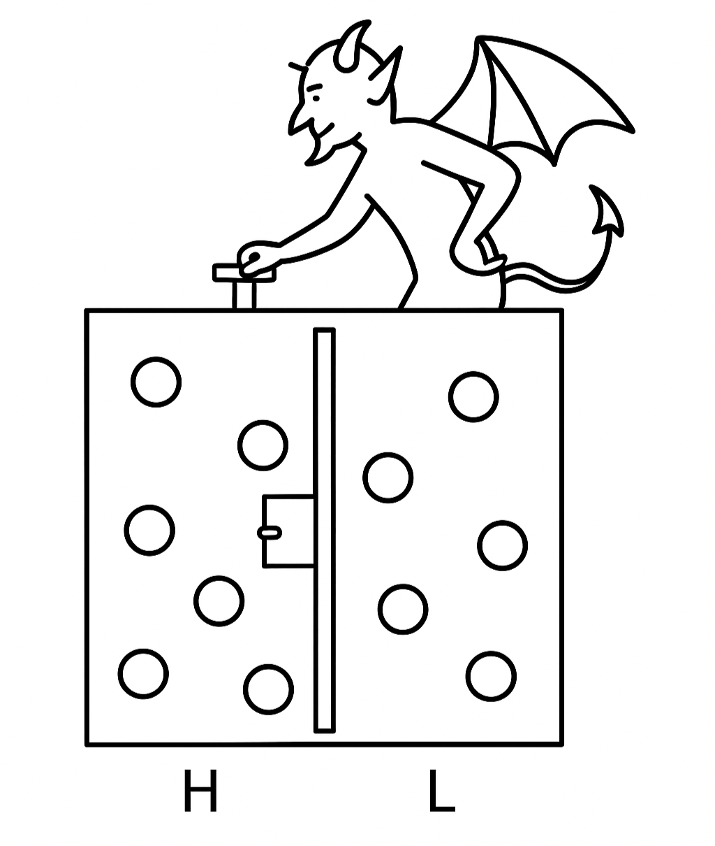
Maxwell did not propose building such a demon; he wanted to probe the foundations of irreversibility. Was the second law truly absolute, or statistical? His thought experiment foreshadowed the probabilistic interpretation later championed by Boltzmann.

3.5.2 Szilard’s Engine

In 1929, Leó Szilard sharpened the paradox with a one-molecule thought experiment. Imagine a cylinder with a single gas particle and a movable piston. Insert a partition, trapping the molecule on one side. By measuring which side the particle occupies, you can allow isothermal expansion that extracts work:

It seems information about the particle’s position has been converted into energy. But where does entropy increase? Szilard argued that the act of measurement must have a thermodynamic cost, hinting that information itself is physical.

3.5.3 Landauer’s Principle: Erasure Costs Heat

In 1961, Rolf Landauer crystallized the resolution: “Information is physical.” He showed that the logically irreversible act of erasing one bit of memory has an unavoidable cost:

The demon can gather information at no thermodynamic cost if done reversibly, but to reset its memory for the next cycle, it must erase. That erasure generates entropy, saving the second law. The paradox dissolves once we include the demon’s memory in the thermodynamic ledger.

3.5.4 Bennett and Reversible Computation

In the 1980s, Charles Bennett of IBM refined this view. He demonstrated that measurement and even computation can, in principle, be performed reversibly without energy cost. The unavoidable step is erasure: discarding information to reuse memory. Thus, the second law survives not in spite of intelligence, but because intelligence itself is bound by physical laws.

3.5.5 Modern Experiments

Advances in nanotechnology have made “demons” real in the lab. Colloidal particles in optical traps, manipulated by feedback control, mimic Szilard’s engine. Experiments confirm the Jarzynski equality and Crooks fluctuation theorem (see §3.8), showing that information can indeed be used as fuel, but always at the cost anticipated by Landauer. No demon escapes entropy; it merely shifts where the bill is paid.

3.5.6 Information Thermodynamics

The lesson is profound: entropy is not merely about energy; it is about information. The microstate of a system contains information, and knowing that information allows extraction of work. But erasing information—forgetting—costs energy. The second law, therefore, is intimately tied to the physics of information processing.

This insight bridges physics and computer science. Every time we erase a file, reset a bit, or clear memory, a minuscule entropy cost is paid. In modern processors, energy dissipation per operation is still orders of magnitude above the Landauer limit, but as devices shrink, this fundamental bound becomes technologically relevant.

3.5.7 Broader Implications

• Biology. Living cells act like Maxwellian demons: molecular machines (enzymes, ion pumps) read and process information to extract work from fluctuations. The coupling of information and thermodynamics is the foundation of life.
• Communication theory. Claude Shannon’s information entropy mirrors thermodynamic entropy: both measure uncertainty. The connection is no accident—Landauer and Bennett closed the conceptual loop.
• Philosophy. Maxwell’s demon illustrates the statistical nature of the second law. Entropy increase is not metaphysical necessity but overwhelming probability once observers and memory are included.

In summary: Maxwell’s demon began as a playful challenge to the second law, but it sparked a revolution. Szilard showed information could be fuel; Landauer showed erasure exacts a thermodynamic cost; Bennett showed reversible computation can sidestep—but not abolish—that cost. Modern experiments confirm that information is physical. The demon did not slay the second law; it revealed its deeper domain, where entropy counts not only energy but also information.

3.6 Boltzmann and Statistical Mechanics

If Clausius gave entropy its name, and Kelvin gave it weight, it was Ludwig Boltzmann (1844–1906) who gave it a soul. His vision was that the second law is not an inviolable commandment but a law of statistics, born of probability. This daring idea—controversial in his lifetime—eventually defined modern physics.

3.6.1 Boltzmann’s Life and Struggles

Born in Vienna, Boltzmann was brilliant, restless, and often embattled. He studied under Josef Stefan, then became professor of theoretical physics. His lectures were electric, but his ideas faced fierce opposition. Many contemporaries rejected the atomic theory; to them, atoms were convenient fictions. Boltzmann staked his career on the reality of atoms and on statistics as the foundation of thermodynamics. The resistance was draining. In 1906, suffering from depression and poor health, he took his own life. On his tombstone in Vienna is carved his most famous equation:

It is both epitaph and triumph: the statistical definition of entropy.

3.6.2 Microstates, Macrostates, and Entropy

Thermodynamics deals with macrostates—descriptions by variables like $(P,V,T,N)$. But each macrostate corresponds to an astronomically large number of microstates, specifying the exact positions and momenta of all particles.

Boltzmann’s key postulate: in equilibrium, all accessible microstates consistent with given constraints (energy $E$, particle number $N$, volume $V$) are equally likely. Then the entropy is proportional to the logarithm of the number of microstates $W$:

Why the logarithm? Because entropy must be extensive: two independent systems should have entropies that add. If system A has $W_A$ states and system B has $W_B$, the combined system has $W_A W_B$ states. Additivity requires

Thus the log is inevitable.

3.6.3 Ensembles and Probability Distributions

Boltzmann’s idea was later refined by Gibbs into ensembles. For a system at fixed $E,N,V$ (the microcanonical ensemble), entropy is

where $\Omega$ counts microstates with energy near $E$.

For a system in contact with a heat bath at temperature $T$ (the canonical ensemble), the probability of microstate $i$ with energy $E_i$ is

Here $Z$ is the partition function, the generator of thermodynamic information:

• Free energy: $F = -k_B T \ln Z$.
• Internal energy: $U = - \partial \ln Z/\partial \beta$.
• Entropy: $S = -k_B \sum_i p_i \ln p_i$.

This bridges microscopic probability with macroscopic thermodynamic potentials.

3.6.4 The H-Theorem

Boltzmann’s boldest stroke was the H-theorem. For a dilute gas, define the single-particle distribution function $f(\mathbf r,\mathbf v,t)$: the probability density of finding a particle near position $\mathbf r$ with velocity $\mathbf v$. Define the functional

Boltzmann’s kinetic equation describes how $f$ evolves due to collisions. Assuming molecular chaos (the Stosszahlansatz: pre-collision velocities are uncorrelated), Boltzmann showed

Thus $H$ decreases monotonically, approaching a minimum at equilibrium. Since entropy $S \sim -k_B H$, entropy increases. The H-theorem provided a microscopic arrow of time: though underlying mechanics are reversible, typical evolution leads toward equilibrium.

3.6.5 Paradoxes and Objections

Boltzmann’s contemporaries raised famous objections.

• Loschmidt’s paradox (reversibility). If we reverse all molecular velocities, the gas would evolve backward, entropy decreasing. How can monotonic increase be fundamental?
  Boltzmann’s reply: Such reversed states are fantastically special; the overwhelming majority of microstates evolve toward higher entropy. The second law is statistical, not absolute.

• Zermelo’s paradox (recurrence). By Poincaré’s recurrence theorem, a finite system will eventually return arbitrarily close to its initial state, implying entropy decrease.
  Reply: True, but recurrence times are unimaginably longer than the age of the universe. For macroscopic systems, recurrence is physically irrelevant.

These debates foreshadowed the modern view: the second law is not ironclad but overwhelmingly probable, its violations negligible for macroscopic systems but detectable in small ones (see §3.8).

3.6.6 Coarse-Graining and Typicality

Why does entropy increase if microscopic dynamics conserve phase-space volume (Liouville’s theorem)? The answer lies in coarse-graining: we cannot track microstates in infinite detail, so we describe them by macrostates (cells in phase space). Under coarse-graining, distributions spread, and entropy increases.

Modern formulations use the concept of typicality: almost all microstates consistent with a macrostate evolve into states corresponding to larger $W$. Entropy increase reflects the fact that low-entropy microstates are vanishingly rare, while high-entropy ones dominate.

3.6.7 Legacy of Boltzmann’s Equation

Boltzmann’s equation,

is the backbone of kinetic theory. It explains viscosity, thermal conductivity, and diffusion. Despite its assumptions, it remains a pillar of nonequilibrium statistical mechanics.

3.6.8 Philosophical and Scientific Impact

Boltzmann’s vision was radical: the laws of thermodynamics are not exceptions to mechanics but statistical consequences. Entropy increase is not absolute necessity but virtual certainty for large systems. This idea resonates through physics:

• Statistical mechanics of critical phenomena. Phase transitions emerge from fluctuations in microstates.
• Quantum statistical mechanics. Entanglement entropy mirrors Boltzmann’s concept.
• Cosmology. The arrow of time reflects initial low entropy and the probabilistic growth thereafter.

In summary: Boltzmann gave entropy its statistical meaning: $S = k_B \ln W$. He explained irreversibility via the H-theorem, faced profound paradoxes, and laid the foundations of modern statistical mechanics. His tragic life underscored the difficulty of pushing radical ideas, but his vision endures. The second law is not a rigid decree but a law of overwhelming probability, arising from the combinatorial vastness of phase space.

3.7 Thermodynamics in Nature and Technology

Thermodynamics is not confined to steam engines and laboratory experiments. Its laws govern clouds and climates, chemical reactions and living cells, turbines and refrigerators. To appreciate the breadth of the discipline, we survey a range of natural and technological arenas where thermodynamic reasoning is decisive.

3.7.1 Phase Equilibria and the Clausius–Clapeyron Relation

When two phases coexist—say, liquid water and vapor—their chemical potentials are equal:

Differentiating this condition yields the Clausius–Clapeyron equation:

where $L$ is the latent heat of transformation and $\Delta v = v_\beta - v_\alpha$ is the specific volume difference between phases. For liquid–vapor transitions, $v_\beta \gg v_\alpha$, so

Approximating vapor as ideal gas and integrating,

This exponential dependence explains why a modest rise in temperature can vastly increase vapor pressure—critical to cloud formation, storm intensification, and boiling phenomena.

Meteorological example. The exponential sensitivity of saturation vapor pressure underlies the Clausius–Clapeyron scaling of atmospheric moisture. A warming climate increases the atmosphere’s water-holding capacity, fueling heavier precipitation events.

3.7.2 Chemical Thermodynamics and Free Energies

The second law governs chemical reactions through the Gibbs free energy $G$.

For a reaction $\sum_i \nu_i A_i = 0$, the Gibbs energy change is

where $\mu_i$ are chemical potentials. At equilibrium,

and the equilibrium constant $K$ is linked to the standard free energy change:

Thus, the spontaneity of reactions depends not on enthalpy or entropy alone but on their balance. Endothermic reactions can proceed if entropy increase outweighs enthalpy cost, and exothermic reactions may stall if entropy decreases too much.

Van ’t Hoff relation. Temperature dependence of equilibrium follows:

This explains why some reactions shift rightward at high $T$ (endothermic) and others leftward (exothermic).

Example. The Haber–Bosch process for ammonia synthesis balances high pressure and moderate temperature to maximize $K$ while maintaining practical kinetics.

3.7.3 Biological Free Energy and Metabolism

Life itself is a thermodynamic phenomenon. Organisms maintain local low entropy by exporting entropy to their environment. The bookkeeping currency is free energy, often carried in molecules like ATP.

• ATP hydrolysis releases about $30\,\mathrm{kJ/mol}$ under cellular conditions. Cells couple unfavorable reactions to ATP hydrolysis so that the combined $\Delta G < 0$.
• Enzymes lower activation barriers, speeding kinetics, but do not change $\Delta G$. They are catalysts, not violators of the second law.
• Ion gradients across membranes act as free-energy reservoirs. The mitochondrial proton gradient powers ATP synthase, a rotary molecular motor that converts electrochemical potential into chemical bonds.
• Information processing in cells echoes Maxwell’s demon: proteins sense molecular states, make decisions, and consume free energy to enforce directionality.

Life demonstrates that the second law is not a sentence of disorder but a condition of existence: to maintain order, systems must consume free energy and increase entropy elsewhere.

3.7.4 Atmospheres and Lapse Rates

Air cools as it rises because expansion against lower pressure requires work. For a dry adiabatic process,

When condensation occurs, latent heat release reduces the lapse rate, producing the moist adiabatic lapse rate, typically $4$–$7\,\mathrm{K/km}$. This stabilizes convection and shapes cloud development.

Thermodynamics thus explains why mountains have snowcaps, why thunderstorms rise to the tropopause, and why global warming alters storm intensities.

Planetary atmospheres. Mars, with thin CO$_2$ atmosphere, shows large diurnal swings; Venus, with dense atmosphere, exhibits a supercritical greenhouse. In each case, thermodynamic principles (radiation balance, adiabatic structure, phase transitions of CO$_2$ or H$_2$O) dictate climate.

3.7.5 Engines, Turbines, and Heat Pumps

Modern technology rests on cycles inspired by Carnot but adapted for practicality.

• Otto cycle (gasoline engines). Efficiency increases with compression ratio but is limited by knock and materials.
• Diesel cycle. Higher compression and temperature ignition yield greater efficiency but heavier engines.
• Brayton cycle (jet engines, gas turbines). Combustion occurs at nearly constant pressure; efficiency rises with pressure ratio and turbine inlet temperature.
• Rankine cycle (steam plants). Adds reheating and regeneration to approach Carnot performance.

Refrigeration exploits the reversed cycles. The coefficient of performance (COP) is bounded by Carnot but degraded by irreversibilities like throttling and finite heat exchanger area.

Exergy analysis. Engineers track where useful work potential is destroyed by irreversibility. In a power plant, the biggest exergy losses occur in combustion and heat transfer across finite $\Delta T$. Identifying these losses guides improvements.

3.7.6 Stability, Response, and Critical Phenomena

Thermodynamics also dictates stability through response functions:

• Isothermal compressibility $$\kappa_T = -\frac{1}{V} \left(\frac{\partial V}{\partial P}\right)_T .$$
• Thermal expansion coefficient $$\alpha = \frac{1}{V} \left(\frac{\partial V}{\partial T}\right)_P .$$

Stability requires $C_P > 0$, $\kappa_T > 0$. Near critical points (e.g., liquid–gas critical point), these quantities diverge, fluctuations become macroscopic, and universality classes emerge. Critical opalescence—milky scattering in near-critical fluids—is entropy fluctuations made visible.

3.7.7 Thermodynamics as a Universal Language

Whether we analyze a thunderstorm, a biochemical pathway, or a turbine blade, the same logic applies:

• Define the system and surroundings.
• Write energy and entropy balances.
• Identify irreversibilities and free-energy sources.

From the microsecond folding of proteins to the billion-year climate of planets, thermodynamics provides the grammar. It is the universal language of transformation.

In summary: Thermodynamics governs the behavior of matter and energy across domains. In phase changes, it sets vapor pressures; in chemistry, it dictates equilibria; in biology, it enables metabolism; in atmospheres, it shapes climate; in machines, it bounds efficiency. The same equations explain boiling water, living cells, and jet engines. The reach of thermodynamics is so vast that it serves not merely as a theory of physics but as a lens through which to view the organization of nature and technology alike.

3.8 Modern Horizons: From Black Holes to the Universe

Thermodynamics, born of steam engines, has expanded its reach to the frontiers of physics: black holes, quantum information, cosmology, and nanoscale systems. The same principles that limited Carnot’s engines now govern the fate of stars, the behavior of molecules, and the arrow of time for the universe itself.

3.8.1 Black-Hole Thermodynamics

In the 1970s, physicists realized that black holes—once thought to be the ultimate entropy sinks—obey laws strikingly similar to thermodynamics.

• Area theorem (Hawking). The surface area $A$ of a black hole’s event horizon never decreases, paralleling the second law.
• Bekenstein entropy. Jacob Bekenstein proposed that a black hole carries entropy proportional to horizon area: $$S_{\text{BH}} = \frac{k_B c^3}{4 G \hbar} A .$$ Astonishingly, entropy is not proportional to volume but to area.
• Hawking radiation. Stephen Hawking showed quantum effects cause black holes to emit thermal radiation, with temperature $$T_H = \frac{\hbar c^3}{8\pi G M k_B}$$ for a Schwarzschild black hole of mass $M$. Black holes are not black but slowly evaporate.

The four laws of black-hole mechanics mirror thermodynamics:

1. Zeroth law. Surface gravity $\kappa$ is constant over the horizon (analogous to uniform temperature).
2. First law. $\mathrm dM = ( \kappa / 8\pi G ) \mathrm dA + \Omega \mathrm dJ + \Phi \mathrm dQ$, linking changes in mass $M$, area $A$, angular momentum $J$, and charge $Q$.
3. Second law. Horizon area never decreases (unless Hawking radiation is included, in which case the generalized entropy $S_{\text{BH}}+S_{\text{outside}}$ never decreases).
4. Third law. It is impossible to reach $\kappa=0$ (absolute zero surface gravity) by finite steps.

Thus, thermodynamics reaches into gravity itself, suggesting spacetime may be emergent from statistical microstates of unknown degrees of freedom.

3.8.2 Fluctuation Theorems and Nanoscale Thermodynamics

At microscopic scales, thermal fluctuations rival averages. The second law still holds on average, but transient violations can occur. These are captured by fluctuation theorems.

• Jarzynski equality (1997).
  For a system driven out of equilibrium by work $W$,

  $$\langle e^{-\beta W} \rangle = e^{-\beta \Delta F},$$

  where $\Delta F$ is the equilibrium free-energy difference. Even far from equilibrium, this exact relation holds.

• Crooks fluctuation theorem.
  The ratio of forward and reverse work distributions is

  $$\frac{P_F(W)}{P_R(-W)} = e^{\beta(W-\Delta F)}.$$

These equalities sharpen the second law. From Jensen’s inequality, Jarzynski’s relation implies $\langle W \rangle \ge \Delta F$, the familiar bound. But the equality itself encodes richer information about fluctuations.

Experiments. Colloidal beads in optical traps, single-molecule pulling (RNA unfolding), and nanoscale electronic devices have verified fluctuation theorems. They show that the second law is not absolute prohibition but a statistical trend, with occasional small violations in tiny systems over short times.

3.8.3 Cosmology and the Arrow of Time

Entropy governs not only engines but also the cosmos. The early universe, moments after the Big Bang, was hot and dense yet surprisingly low in gravitational entropy—nearly uniform matter with tiny fluctuations. Smoothness corresponds to fewer gravitational microstates than clumpy configurations (stars, galaxies, black holes). Thus, the universe began in a very special state of low entropy.

As time progresses, gravitational clumping increases entropy: galaxies form, stars ignite, black holes grow. The arrow of time—our sense of past and future—emerges from this low-entropy beginning.

Heat death? If expansion continues indefinitely, the universe may approach a state of thermal equilibrium: stars burn out, black holes evaporate, and entropy reaches a maximum. But with dark energy driving accelerated expansion, the ultimate fate may be more exotic—an ever-colder, ever-emptier cosmos.

Cosmic microwave background (CMB). The near-uniformity of the CMB encodes the low-entropy initial condition. Without such special beginnings, the universe would not have the thermodynamic “room” to evolve complexity.

3.8.4 Quantum Thermodynamics and Information

Quantum mechanics reshapes thermodynamics when coherence and entanglement matter.

• Resource theories. Quantum thermodynamics treats states and operations under constraints (thermal contacts, unitaries). Free energies generalize to whole families indexed by Rényi entropies.
• Quantum engines. Three-level masers and qubits can serve as working media. Efficiency is still bounded by Carnot, but coherence and correlations act as new resources.
• Entanglement entropy. In quantum many-body systems, entanglement provides a statistical measure akin to thermodynamic entropy. Black-hole entropy may reflect entanglement between inside and outside degrees of freedom.
• Quantum information. Landauer’s principle persists: erasing a qubit’s state costs $k_B T \ln 2$. Quantum error correction thus carries a thermodynamic price tag.

Experiments. Superconducting qubits, trapped ions, and NV centers in diamond realize quantum heat engines, testing the interplay of coherence and dissipation.

3.8.5 Toward Emergent Laws

That thermodynamics applies from atoms to galaxies hints at universality. Some theorists propose that spacetime itself is a thermodynamic construct, arising from coarse-grained microstates of unknown origin. The holographic principle, black-hole entropy, and AdS/CFT duality all suggest a deep link between information and geometry.

In summary: Modern horizons of thermodynamics stretch from black holes emitting Hawking radiation to molecules fluctuating under optical tweezers. Fluctuation theorems refine the second law; cosmology frames the arrow of time; quantum engines and entanglement extend free-energy concepts. Thermodynamics, born of pistons and boilers, now writes the rules of the cosmos and the quantum.

3.9 Conclusion: The Legacy of Thermodynamics

Thermodynamics began with furnaces and engines, but it became a universal language of order and change. It tells us not only what can happen but what cannot. In doing so, it established boundaries that shape both technology and our understanding of the cosmos.

3.9.1 The Four Laws in Perspective

• Zeroth law. Temperature is meaningful and transitive: if A is in equilibrium with B, and B with C, then A with C. This simple observation grounds the concept of thermometers and defines temperature scales.

• First law. Energy is conserved. The law rules out perpetual motion of the first kind and gives us the accounting to track heat, work, and internal energy.

• Second law. Entropy of an isolated system never decreases. This is the arrow of time, the reason engines cannot be perfect, the principle that milk does not unspill.

• Third law. As $T \to 0$, entropy approaches a constant minimum. Absolute zero is unattainable in finite steps. This anchors cryogenics and quantum ground states.

Together, these laws are as universal as Newton’s laws, yet broader: they govern chemistry, biology, information, and gravity itself.

3.9.2 Intellectual Legacy

Thermodynamics transformed physics in three ways:

1. From determinism to probability. Boltzmann showed that macroscopic irreversibility arises from microscopic reversibility by overwhelming probability. The second law is statistical, not absolute.

2. From mechanics to information. Maxwell’s demon and Landauer’s principle revealed that entropy counts not only energy but information. Erasing memory costs heat. Thermodynamics thus underpins computation and communication.

3. From engines to the universe. The discovery of black-hole entropy and Hawking radiation expanded thermodynamics to spacetime itself. What began with pistons now governs horizons.

3.9.3 Practical Legacy

• Technology. Thermodynamics powers turbines, refrigerators, semiconductors, and chemical plants. Efficiency benchmarks like Carnot’s theorem still guide design. Exergy analysis identifies waste and optimizes sustainability.

• Biology. Life is a thermodynamic enterprise. Organisms export entropy to maintain order. Metabolism, ATP, and molecular machines are all expressions of free-energy management.

• Climate and Earth systems. From the moist lapse rate to the water cycle, climate is a thermodynamic engine driven by the Sun. Understanding entropy flows is key to predicting and mitigating climate change.

• Information technology. As transistors shrink, the Landauer bound becomes relevant. Thermodynamics now constrains not only power plants but microprocessors.

3.9.4 Philosophical Resonance

Thermodynamics speaks to deep questions:

• Why does time have a direction? Because entropy increases.
• Why does order exist? Because systems can maintain local order by exporting entropy.
• What is the fate of the universe? Possibly heat death, as entropy climbs toward its maximum.

Arthur Eddington captured its authority: “If your theory is found to be against the second law of thermodynamics, I can give you no hope.” Few statements in science carry such weight.

3.9.5 Looking Forward

In the 21st century, thermodynamics continues to evolve:

• Nanoscale physics. Fluctuation theorems extend the second law to small systems.
• Quantum thermodynamics. Entanglement and coherence introduce new resources, but Carnot bounds persist.
• Cosmology. Entropy frames the arrow of time and the role of initial conditions in the universe’s evolution.

Thermodynamics is thus unfinished: it remains the template by which new domains are measured.

In summary: Thermodynamics is more than a science of heat. It is the science of limits—of what can and cannot be done. From Carnot’s engines to Boltzmann’s probabilities, from Maxwell’s demon to Hawking’s radiation, it traces a single thread: energy is conserved, entropy grows, and order is precious and costly. The legacy of thermodynamics is universal: it powers our machines, shapes our lives, and sets the terms of the universe itself.