6 Early quantum theory

6.1 Introduction: Cracks in the Classical Edifice

By the end of the 19th century, physics flexed like it had the final boss down. Newtonian mechanics ruled motion, Maxwell’s equations ruled fields, thermodynamics ruled heat. Yet precision experiments began posting L’s for classical theory. A new playbook—quantum—was loading.

What broke first? Three pillars:

1. Radiation and heat. The spectrum of an ideal glowing cavity (a blackbody) refused to follow classical predictions. Equipartition and Maxwell’s waves led to infinite ultraviolet energy—an “ultraviolet catastrophe.”

2. Light and electrons. Shining light on a clean metal knocked out electrons with sharp rules that defied wave-only intuition.

3. Atoms and spectra. Gases glowed at razor-thin frequencies described by simple formulas, yet any classical electron orbiting a nucleus should radiate and spiral inward.

These cracks weren’t edge cases; they were mainstream physics behaving weirdly.

6.1.1 Characters entering the stage

Max Planck (1900). A thermodynamics purist backed into heresy. To fit blackbody data, he quantized energy exchange in chunks of $h\nu$. He thought it was a mathematical trick; the universe took him literally.

Albert Einstein (1905). The “patent-clerk energy.” He said the quiet part out loud: light itself comes in quanta (photons). With that, the photoelectric rules suddenly made sense, and $E=h\nu$ stepped out of the blackbody and into matter.

Ernest Rutherford (1911). He yeeted Thomson’s “plum pudding” and installed a nuclear atom after alpha particles bounced at wild angles from gold foil. But a classical electron racing around a tiny nucleus should radiate energy and crash. Stable atoms? Not in classical land.

Niels Bohr (1913). He proposed that electrons live only on special orbits with quantized angular momentum and jump between them by absorbing or emitting light at specific frequencies. The hydrogen spectrum clicked into place—partial victory, but weird rules demanded deeper logic.

Louis de Broglie (1923–24). If light acts like particles, maybe matter acts like waves. He proposed $\lambda=h/p$, a hypothesis begging for an experiment.

6.1.2 The “classical no-go”s (with minimal math)

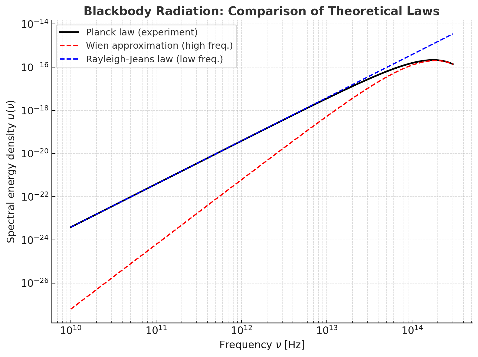
Blackbody catastrophe. Classical equipartition feeds every electromagnetic cavity mode an average energy $k_B T$. Counting modes yields a spectral energy density that rises $\propto \nu^2$, blowing up at high frequency. Data said “nope”—the spectrum peaks and falls.

We will show in §6.2 that introducing energy quanta leads to Planck’s distribution and cures the divergence

No ultraviolet apocalypse appears in this curve

Photoelectric rules. Experiments found: (i) no electrons below a threshold frequency, however intense the light, (ii) above threshold, the maximum electron kinetic energy is linear in frequency, not intensity, (iii) emission is effectively instantaneous. Einstein’s one-liner,

nailed it, where $W$ is the work function. Intensity controls how many photons hit, not their individual energy

Atomic spectra. Balmer and Rydberg wrote beautiful empirical formulas for hydrogen lines. Rutherford’s nuclear atom raised the stakes: a tiny, charged nucleus should make orbiting electrons radiate continuously and smear the spectrum—contradiction. Bohr’s move was to quantize angular momentum and energy levels, producing discrete lines and a frequency rule that matched Rydberg’s data. But why those orbits? Old quantum theory worked, then stalled.

6.1.3 The vibe: discrete meets wave

The early quantum story is a series of “wait, both?” moments:

• Light interferes like a wave but trades energy like a particle
• Electrons behave like particles in tracks yet diffract like waves through crystals
• Energy in atoms is not continuous real estate; it’s a floor plan of levels with allowed transitions

The common thread is discreteness sneaking into systems previously modeled as continuous. That discreteness shows up in spectra, specific heats, threshold effects, and stability.

6.1.4 Minimal mathematical promises (to be delivered in later sections)

• Planck spectrum. From counting quanta with weight $\exp(-nh\nu/k_B T)$ we will derive the energy density above and recover the Stefan–Boltzmann law and Wien’s displacement

• Einstein photoelectric equation. Straight line plots of $K_{\max}$ vs $\,\nu$ give slope $h$ and intercept $W$—that is how early experiments measured Planck’s constant with electrons

• Bohr energies. For hydrogen-like atoms we will get

and the emitted photon frequency from a jump $n\to n'$ will satisfy $h\nu = E_n - E_{n'}$ with Rydberg constant emerging naturally

• de Broglie hypothesis. Assuming $p=h/\lambda$ and $E=h\nu$ makes group velocity match particle velocity and predicts electron diffraction, later seen in labs

6.1.5 What “early quantum theory” is (scope note)

We will live mostly in 1900–1925: the old quantum theory (Planck → Einstein → Bohr–Sommerfeld → de Broglie) and its decisive experiments (Franck–Hertz, Davisson–Germer, Stern–Gerlach). Full quantum mechanics (Heisenberg’s matrices and Schrödinger’s waves, 1925–26) is the bridge to the next chapter, but we will aim the runway here: when classical intuition finally yields and a consistent quantum calculus becomes inevitable.

6.2 Blackbody Radiation and Planck’s Hypothesis

Blackbody radiation is where classical physics face-planted and quantum theory quietly spawned. A blackbody is an ideal cavity with a tiny hole: light that enters bounces around and is essentially absorbed; light that leaves carries the equilibrium spectrum of the cavity walls. The mission in the 1890s was to predict the energy density of this radiation as a function of frequency $\nu$ and temperature $T$ and to explain why the measured curve rises, peaks, and then crashes instead of diverging. Spoiler: classical equipartition said “infinite UV energy,” nature said “lol, no,” and Max Planck invented quanta to get the curve right.

6.2.1 The experimental scene: precision burns theory

German labs (Lummer, Pringsheim, Rubens, Kurlbaum) built exquisitely calibrated cavities and detectors. At moderate and high frequencies, the data followed Wien’s law remarkably well; at low frequencies (long wavelengths), new measurements started to bend away from Wien’s exponential falloff, demanding a better formula. Planck followed these plots obsessively—enough that when Rubens showed him fresh long-wavelength data in October 1900, he went home and cooked up the curve that matched everything.

Two common ways to describe the spectrum are by frequency and by wavelength. They are related but not identical in shape because $\nu=c/\lambda$ changes the measure:

You’ll see two standard forms. By frequency:

By wavelength:

We’ll derive $u_\nu$ first and then convert to $u_\lambda$.

6.2.2 Mode counting in a cavity: the $8\pi \nu^{2}/c^{3}$ factor

Take a cubic cavity with perfectly conducting walls. Electromagnetic standing waves fit only certain wavevectors $\boldsymbol k$; each allowed mode is a harmonic oscillator. Counting modes with frequencies between $\nu$ and $\nu+d\nu$ gives a density of states per unit volume

The $8\pi$ comes from spherical shells in $\boldsymbol k$-space and from two polarization states. This factor is pure geometry/kinematics and will be the same in classical and quantum derivations. The physics enters when we decide how much average energy to assign to each mode at equilibrium.

6.2.3 Classical attempt: equipartition and the ultraviolet catastrophe

In classical statistical mechanics, every quadratic degree of freedom contributes $\tfrac{1}{2}k_B T$ to the mean energy. A harmonic oscillator (one mode) has two quadratic pieces (potential and kinetic), so the mean energy per mode would be

Multiply by the mode density to get the spectral energy density

This is the Rayleigh–Jeans law. It works at low frequencies but skyrockets as $\nu^{2}$ and, when integrated over all frequencies, diverges. That divergence—the ultraviolet catastrophe—is not a cute nickname; it is classical physics predicting infinite energy in any warm room. Reality declines.

6.2.4 Wien’s law: a great half-truth

Empirically, Wien proposed

with constants $A,B$ fit to data. This law nails the high-frequency tail (it decays exponentially) and implies the correct displacement law (the peak slides linearly with $T$), but it fails at low frequencies, where experiments show $u_\nu\propto \nu^{2}T$ (Rayleigh–Jeans behavior), not $\nu^{3}$. In short, Wien gets the UV, Rayleigh–Jeans gets the IR, and neither gets the full mixtape.

6.2.5 Planck’s move: discretize the energy exchange

Planck’s radical idea was to treat the cavity walls as a set of microscopic oscillators (resonators) that exchange energy with the radiation field in discrete packets of size $h\nu$:

Given Boltzmann weights, the partition function for one oscillator of frequency $\nu$ is

The mean energy per oscillator is then

Multiply by the density of modes $g(\nu)$ to get the full spectrum:

This is Planck’s law, 1900. It reduces to Rayleigh–Jeans at low frequency (expand the exponential) and to Wien’s exponential at high frequency. One curve to rule them all.

6.2.6 Low- and high-frequency limits (sanity checks)

Let $x \equiv h\nu/(k_B T)$.

• Low frequency ($x\ll 1$): $e^{x}-1 \approx x$, so

which is Rayleigh–Jeans

• High frequency ($x\gg 1$): $e^{x}-1 \approx e^{x}$, so

which is Wien’s law with $A=8\pi h/c^{3}$ and $B=h/k_B$

So Planck’s formula gracefully bridges the two regimes that classical and empirical laws captured separately.

6.2.7 Total energy and Stefan–Boltzmann law

Integrate $u_\nu$ over all frequencies to get the total energy density $u(T)$:

Change variables $x=h\nu/(k_B T)$; then $d\nu = (k_B T/h)\,dx$ and

The integral is a famous one:

So

The radiated power per unit area from a black surface follows by $I=\tfrac{c}{4}u$ (kinematic factor for isotropic radiation):

This is the Stefan–Boltzmann law with its constant $\sigma$ expressed in terms of $k_B,h,c$.

6.2.8 Where is the peak? Wien’s displacement law

Maximize $u_\nu(\nu,T)$ with respect to $\nu$ at fixed $T$. Setting $x=h\nu/(k_B T)$, the condition reduces to

This transcendental equation has a root

Hence the frequency of the peak scales as

If you instead work with the wavelength form

and maximize with respect to $\lambda$, you get Wien’s displacement law

with a constant $b$ fixed by the root of a slightly different transcendental equation. Important PSA: the peak in $u_\nu$ and the peak in $u_\lambda$ are not at the same photon energy because the Jacobian $|d\nu/d\lambda|$ reshapes the curve.

6.2.9 Converting between frequency and wavelength spectra

Use $u_\lambda\,d\lambda = u_\nu\,d\nu$ with $\nu=c/\lambda$ and $d\nu = -\,c/\lambda^{2}\,d\lambda$. Then

Plugging Planck’s $u_\nu$ gives the standard $u_\lambda$ quoted above. The minus sign drops because decreasing $\lambda$ increases $\nu$.

6.2.10 A statistical-mechanics view (why quantization matters)

Classically, energy is continuous and equipartition dumps $k_B T$ into each mode no matter how high its frequency. Quantum statistically, the occupation of a mode with energy spacing $h\nu$ is Bose–Einstein with zero chemical potential:

and the mean energy per mode is $h\nu\,\bar n(\nu)$. High-frequency modes are exponentially hard to populate because you must pay $h\nu$ upfront; low-frequency modes behave classically because $h\nu \ll k_B T$ makes $\bar n$ large and $\langle \varepsilon \rangle \to k_B T$. The catastrophe disappears because discrete energy spacing throttles the UV.

6.2.11 Planck’s “I didn’t mean to be a revolutionary” arc

Planck was a dyed-in-the-wool thermodynamics guy who wanted a principled derivation of Wien’s empirical law. After the Rubens data contradicted Wien at low $\nu$, he sought an interpolation that matched both limits and then reverse-engineered a statistical story to justify it. He later called the quantization step “an act of desperation.” The act stuck. Within five years Einstein gave those energy packets—photons—independent life in the photoelectric effect. Planck’s constant $h$ went from curve-fitting fudge to a fundamental unit of nature.

6.2.12 Practical knobs: emissivity and real surfaces

Real materials are not perfect blackbodies. If a surface has emissivity $\epsilon(\nu,T)$ between 0 and 1, its spectral radiance is

Kirchhoff’s law of thermal radiation says emissivity equals absorptivity at each frequency, so cavities with a small aperture are effectively black even if the walls are not—rays bounce until they hit an absorptive patch. This is why laboratory blackbodies are cavities.

6.2.13 Worked mini-examples

(a) Power of a star. Approximating a star as a blackbody of radius $R$ and surface temperature $T$, its luminosity is

(b) Peak color of a filament. Using $\lambda_{\text{peak}}\,T=b$, heating a filament so $T$ doubles halves the peak wavelength, shifting from red toward blue. Photographs feel the shift because camera sensors respond to $u_\lambda$ weighting.

(c) Cavity photon number density. The photon number spectrum is $n_\nu = u_\nu/(h\nu)$, hence the total number density is

Changing variables $x=h\nu/(k_B T)$ yields $n(T)\propto T^{3}$ with a proportionality constant involving $\zeta(3)$.

6.2.14 What to remember (exam-tier TL;DR)

• Geometry gives the density of modes $g(\nu) = 8\pi \nu^{2}/c^{3}$; physics gives the average energy per mode
• Classical equipartition $\Rightarrow$ Rayleigh–Jeans $\propto \nu^{2}T$ $\Rightarrow$ ultraviolet catastrophe
• Planck: energy exchange in quanta $h\nu$ $\Rightarrow$ $\langle \varepsilon \rangle = h\nu/(e^{h\nu/(k_B T)}-1)$
• Multiply them to get Planck’s law; integrate to get Stefan–Boltzmann $I=\sigma T^{4}$; maximize to get Wien’s displacement
• Quantization is not optional decoration; it is the only way to make thermodynamics and electromagnetism coexist peacefully in a cavity

6.3 Photoelectric Effect and Einstein’s Light Quanta

Shine light on a clean metal and electrons pop out. Classical waves could explain “more light → more energy,” but experiments in the early 1900s said “frequency first, intensity second.” That plot twist pushed Einstein to a bold take: light energy arrives in discrete packets of size $h\nu$. The photoelectric effect is where photons stop being poetry and start being accounting.

6.3.1 The experimental rules (what needed explaining)

Laboratories found a crisp set of facts:

• There exists a threshold frequency $\nu_0$ below which no electrons are emitted, however intense the light
• Above threshold, the maximum kinetic energy of emitted electrons depends linearly on frequency, not intensity
• The emission is prompt on the scale of the light cycle; no measurable delay even at low intensities
• The photoelectric current (number of electrons per second) scales with light intensity for fixed frequency, up to a saturation set by the apparatus

These rules are weird in a pure wave picture where energy is spread out over the wavefront and can accumulate continuously.

6.3.2 Einstein’s one-liner

Einstein’s 1905 hypothesis: light of frequency $\nu$ behaves as a stream of quanta (photons), each carrying energy $h\nu$. An electron in the solid that absorbs one photon spends part of that energy to escape the material—this is the work function $W$—and keeps the rest as kinetic energy. Thus

The threshold frequency is therefore

Intensity controls how many photons arrive per second, hence how many electrons can be emitted per second, but not the maximum energy of each electron. Frequency sets the budget per electron.

6.3.3 Measuring $h$ and $W$ with stopping potentials

Experimenters measure the maximum kinetic energy by applying a retarding voltage $V_s$ to stop the most energetic electrons from reaching the collector. The definition is

Combining with Einstein’s relation gives a straight-line plot

So a graph of $V_s$ versus $\nu$ has slope $h/e$ and intercept $-W/e$. That is how early experiments extracted Planck’s constant and the work function directly from electron kinetics.

6.3.4 Why the classical wave picture face-plants

A classical wave deposits energy continuously at a rate proportional to intensity. If that were the whole story, then at low intensities electrons should need a long time to accumulate enough energy to escape (a measurable delay), and for sufficiently intense low-frequency light the effect should happen anyway—no threshold. Neither occurs. The data scream “energy arrives in lumps,” with each electron grabbing at most one lump.

6.3.5 Millikan’s reluctant confirmation

Robert Millikan spent a decade trying to break Einstein’s interpretation by doing gold-standard measurements. He refined vacuum systems, surface preparation, and electronics. The result was the cleanest straight lines in physics: $eV_s$ versus $\nu$ with slope $h$ and a frequency intercept at $W/h$. Millikan didn’t like the photon idea philosophically, but his data left no wiggle room. If your enemy measures your theory and it wins, that’s a W.

6.3.6 From intensity to flux: how many electrons?

Hold $\nu$ fixed above threshold. Doubling intensity doubles the photon flux at the surface. If the surface is clean and space-charge effects are controlled, the saturation current $I_{\text{sat}}$ scales linearly with intensity because each absorbed photon can liberate at most one electron. The fraction that actually escape is the quantum efficiency $\eta$; thus

where $P$ is the optical power absorbed on the active area. Real values of $\eta$ depend on the material, surface state, and whether photoelectrons are backscattered or trapped before reaching the collector.

6.3.7 Energy distribution and the role of the solid

$K_{\max}$ is the upper edge. The distribution of kinetic energies depends on the band structure and scattering within the solid. In simple metals one can sketch an “initial state” between the Fermi level and a few $k_B T$ below it; an electron that absorbs a photon emerges with energy roughly $h\nu - W$ minus any losses to inelastic scattering on the way out. That is why measured spectra are broad, not delta functions, even though the top edge follows $h\nu - W$ cleanly.

6.3.8 Time-of-flight and “instantaneous” emission

Modern fast electronics confirm the old claim: emission is prompt within picoseconds or faster, consistent with a single-photon process instead of a long integration. In photon language, a single absorption event transfers $h\nu$ in one go; there is no need to “wait” for energy to build up.

6.3.9 Surface physics and work function engineering

The work function $W$ is a surface property: it depends on the material, crystal face, cleanliness, and adsorbates. Alkali metals with low $W$ respond to red light; clean noble metals require blue/UV. Coatings and cesiation can lower $W$, tuning $\nu_0=W/h$ downward. This is why phototubes and photocathodes care deeply about surface preparation.

6.3.10 Typical lab analysis workflow

1. Illuminate a freshly prepared metal surface with monochromatic light at several frequencies
2. For each $\nu$, sweep the collector voltage negative until the photocurrent drops to zero to find $V_s$
3. Plot $eV_s$ versus $\nu$; fit a line to extract slope $h$ and intercept $-W$
4. Independently, measure saturation current versus intensity at fixed $\nu$ to confirm linear scaling of electron count with photon flux

The two experiments probe different pieces of Einstein’s model: the energy per photon and the counting of photons.

6.3.11 What about intensity at fixed frequency?

At fixed $\nu>\nu_0$, increasing intensity raises the number of emitted electrons (current) but leaves the maximum energy unchanged because $h\nu$ is unchanged. Conversely, at fixed intensity, increasing frequency raises $K_{\max}$ linearly. On the $V_s$–$\nu$ plot, intensity just changes how quickly you reach saturation, not the slope or intercept.

6.3.12 Photons, momentum, and consistency checks

Photons also carry momentum $p=h/\lambda$. In photoemission from a flat surface, most of the photon momentum is small compared with electron Fermi momenta, so $p$ is less central than $h\nu$ for escape energetics, but radiation pressure and light-driven forces make sense in the same bookkeeping. Later phenomena—Compton scattering of X-rays—extend the particle-like picture by showing wavelength shifts that require both photon energy and photon momentum conservation. The photoelectric effect is the gentle on-ramp; Compton is the highway.

6.3.13 Why “one photon → one electron” has caveats

At high intensities and short pulses, multi-photon photoemission can occur: two (or more) photons combine to eject an electron even when $h\nu$ is below $W$. The signature is a nonlinear dependence of current on intensity. The original continuous-wave experiments lived in a regime where the single-photon process dominates, which is why Einstein’s linear law described them. Quantum mechanics contains both regimes—you just move along the intensity axis.

6.3.14 Quick derivations you can do on a napkin

Threshold. Set $K_{\max}=0$ in Einstein’s law to get $\nu_0=W/h$. This is the cleanest way to define $W$ experimentally with light.

Slope extraction. From $eV_s=h\nu - W$, the slope of $V_s$ vs $\nu$ is $h/e$. Measure it and you have a value of $h$ independent of blackbody fits or spectroscopy.

Work function units. If $W$ is reported in electron-volts, then the threshold in hertz is

and in wavelength

It is common to quote $\lambda_0$ for a photocathode because engineers think in wavelengths.

6.3.15 Photoelectric devices: from bench to tech

• Vacuum photodiodes and photomultipliers. Use photoemission from a low-$W$ cathode to seed electrons, then multiply via dynodes. The $V_s$ method turns into gain calibration and noise analysis
• Solar cells (not the same effect). Photovoltaic junctions convert light to electricity via electron–hole pairs and built-in fields, not vacuum photoemission, but the $h\nu$ threshold idea still sets which photons can be absorbed
• Ultrafast electron sources. Femtosecond lasers drive single- or few-photon emission to produce short electron bunches for diffraction and microscopy

6.3.16 Conceptual audit

• Particle-like energy transfer. $h\nu$ per photon, one photon per primary electron escape event
• Material gatekeeper. The work function $W$ sets the doorway; $\nu_0=W/h$ is the key frequency
• Linear edge. $K_{\max}$ tracks $h\nu-W$ regardless of intensity; stopping potential nails it as $eV_s$
• Counting vs energy. Intensity changes how many electrons, frequency changes how energetic they can be

Quantum takes the wheel precisely where classical physics insists on the wrong dependencies.

6.4 Atomic Spectra and Bohr’s Model

Spectral lines were the OG QR codes of atoms—thin, repeatable, and screaming “there’s structure in here.” Long before quantum mechanics became a full theory, careful spectroscopy mapped those lines into simple integer patterns. The old quantum theory’s biggest W was Bohr’s 1913 model: a semi-classical atom with quantized orbits that nailed hydrogen’s spectrum and hinted at a deeper wave picture.

6.4.1 Empirical prelude: Balmer–Rydberg patterns

Hydrogen’s visible lines fit Balmer’s 1885 formula; Rydberg soon generalized it to a wavenumber series

Here $R$ is the Rydberg constant and $(n_i,n_f)$ are positive integers labeling initial and final “levels.” Famous series:

• Lyman $n_f=1$ (ultraviolet)
• Balmer $n_f=2$ (visible; Hα is $n_i=3\to2$ at $\sim 656\,$nm)
• Paschen $n_f=3$ (infrared)

These were pure numerology—but spookily consistent across gases once you inserted effective constants.

6.4.2 Rutherford’s atom and the classical fail

Rutherford’s 1911 scattering showed a tiny, charged nucleus. Classical electrons orbiting such a nucleus are accelerated charges; Maxwell says they radiate and spiral in. That predicts continuous spectra and no stable atoms. Yet nature flexed discrete lines and stability. Enter Bohr.

6.4.3 Bohr’s postulates

Bohr’s model stapled three rules onto classical mechanics:

1. Stationary states. Certain orbits are allowed and do not radiate despite acceleration
2. Quantum of action. Angular momentum is quantized

3. Frequency condition. Radiation occurs only when jumping between stationary states, with photon energy

These hacks were audacious—and shockingly predictive for one-electron atoms.

6.4.4 Coulomb plus quantization: solving for radii, speeds, energies

For a nucleus of charge $+Ze$ and an electron in a circular orbit of radius $r$ and speed $v$, centripetal force equals Coulomb attraction

Combine with the quantization $m_e v r = n\hbar$ to eliminate $v$ and solve for $r_n$:

The bracket is the Bohr radius

so $r_n = \dfrac{n^{2}}{Z}\,a_0$. The orbital speed follows as

where

is the fine-structure constant. The total energy is kinetic plus potential

which evaluates to

For hydrogen ($Z=1$), the ground state is

and levels scale like $-13.6\,\text{eV}/n^{2}$.

6.4.5 From Bohr levels to the Rydberg formula

Bohr’s frequency condition with $E_i$ and $E_f$ gives a photon wavenumber

Thus the Rydberg constant in the infinite nuclear mass limit is

For real hydrogen, the electron orbits the center of mass; replace $m_e$ by the reduced mass

to get

This tiny correction produces isotope shifts between H and D.

6.4.6 Why $m v r = n\hbar$ felt less random over time

A decade later, de Broglie proposed matter waves with $\lambda = h/p$. Demanding an integer number of wavelengths around a circular orbit,

implies

i.e., Bohr’s rule. The standing wave picture explains why only certain radii are stable: destructive interference kicks out the rest. This wave logic is what Schrödinger will formalize in Chapter 7.

6.4.7 Correspondence principle and large $n$

Bohr insisted that for large quantum numbers, quantum predictions must approach classical results. For $n\gg1$, the orbital frequency of the electron matches the emission frequency between neighboring levels, and the pattern of allowed transitions mimics the classical Fourier components of a Coulomb orbit. This “correspondence principle” guided the old quantum theory when full mechanics was still loading.

6.4.8 Selection rules and intensities (why some lines are strong)

Bohr’s model locates levels but doesn’t compute line intensities. Empirically, strong lines obey angular-momentum-like selection rules such as $\Delta l=\pm 1$ that later emerge from dipole transition matrix elements in wave mechanics. The old theory guessed at them via classical radiation patterns; quantum mechanics derives them cleanly.

6.4.9 Worked mini-derivations

(a) Lyman-α wavelength. From $n_i=2\to n_f=1$,

so

Numerically this lands near $121.6\,$nm once $\mu$ is included.

(b) Balmer Hα line. For $n_i=3\to n_f=2$,

so

which evaluates to about $656.3\,$nm.

(c) Ionization energy from level $n$. Send $n\to\infty$; the needed energy is

for hydrogen.

6.4.10 Sommerfeld’s ellipses and early fine structure

To push further, Sommerfeld allowed elliptical orbits and quantized both the radial and angular actions. Adding a relativistic mass–velocity correction produced a partial account of fine structure (small level splittings) and the anomalous spacing of closely lying lines. It was clever but messy, and ran out of road on multi-electron atoms and precision details.

6.4.11 Where Bohr wins, where it breaks

Wins

• Predicts $E_n \propto -1/n^{2}$ and the exact hydrogen and hydrogenic spectra when reduced mass is included
• Explains series limits and ionization energies
• Anticipates de Broglie and provides a clean bridge to wave mechanics

Breaks

• Cannot explain line intensities and polarizations from first principles
• Fumbles fine structure fully and the Zeeman effect anomalies
• Faceplants on helium and other multi-electron atoms
• Treats non-radiating “accelerated” electrons by fiat rather than mechanism

These failures are not bugs—they are breadcrumbs pointing to a wave equation and spin.

6.4.12 Practical constants and forms you will use

Equivalent and handy expressions:

For a hydrogenic ion with nuclear charge $Z$, replace $R_{\text{H}}$ by $Z^{2} R_{\text{H}}$ and $E_n$ by $-13.6\,Z^{2}\,\text{eV}/n^{2}$.

6.4.13 Concept check: Bohr vs wave mechanics

Bohr’s radii $r_n$ correspond to maxima in the radial probability density of the exact hydrogen wavefunctions. The quantum number $n$ remains, but $l$ and $m$ split levels and determine shapes; stationary states become standing waves in three dimensions. The photon frequency condition survives as energy eigenvalue differences, while selection rules arise from matrix elements of the dipole operator.

6.4.14 Minimal problem kit

• Derive $r_n$ and $E_n$ from force balance plus $m v r=n\hbar$ and check $a_0$ numerically
• Starting from $E_n$, recover the Rydberg formula and identify $R_\infty$ in terms of $\alpha$
• Include the reduced mass and estimate the H–D isotope shift of Hα
• Use $v_n=Z\alpha c/n$ to check nonrelativistic consistency ($v_1\approx \alpha c$ for H)

6.5 Rutherford Scattering and the Nuclear Atom

Sometimes one experiment deletes an entire worldview. The Geiger–Marsden gold-foil experiment did exactly that. They fired alpha particles (helium nuclei) at an ultra-thin gold foil and counted scintillations on a screen. Most alphas zipped through with tiny deflections, but a surprising few bounced at large angles, even backward. If positive charge were smeared throughout the atom (Thomson’s “plum pudding”), big-angle kicks would be essentially impossible. The data demanded a concentrated, tiny, positively charged nucleus.

6.5.1 What was measured and why it shocked people

• Beam: alpha particles around a few MeV
• Target: sub-micron gold foil, atomic number $Z=79$
• Detector: zinc sulfide screen counting single scintillations
• Surprise: an exceedingly small fraction scattered through tens of degrees or more, some near $180^\circ$

Classically, if positive charge were diffuse, only small, cumulative nudges add up. Large-angle events practically require a short-range, strong encounter with a compact center—i.e., a nucleus.

6.5.2 Coulomb repulsion and hyperbolic orbits

Treat the interaction as repulsive Coulomb between an alpha of charge $z e$ (with $z=2$) and a nuclear charge $+Ze$:

It is convenient to define

Nonrelativistic trajectories are hyperbolae. The relation between scattering angle $\theta$ and impact parameter $b$ for a projectile of kinetic energy $E$ is

which inverts to

Here $E=\tfrac{1}{2}\mu v^2$ with reduced mass $\mu$; for a very heavy target, $\mu\approx m_{\alpha}$ and lab $\approx$ CM.

6.5.3 The Rutherford differential cross section

The measurable is the angular distribution, i.e. the differential cross section:

Using $b(\theta)$ above and $db/d\theta = -\tfrac{k}{4E}\csc^2(\theta/2)$ gives the famed Rutherford formula

Key scalings:

• $\propto Z^{2} z^{2}$, so heavier nuclei punch harder
• $\propto E^{-2}$, so higher beam energy suppresses scattering
• Diverges at small angles like $\theta^{-4}$

That $1/\sin^{4}(\theta/2)$ falloff matches the data over a wide range—until other physics (screening, nuclear forces, relativity) kicks in.

6.5.4 Distance of closest approach and nuclear scale

For head-on approach ($b=0$, $\theta=\pi$) the kinetic energy converts into potential energy at the turning point $r_{\min}$:

so

Numerically, the handy constant is $e^{2}/(4\pi\varepsilon_{0}) \approx 1.44\ \text{eV}\cdot\text{nm}$. For $z=2$ alphas on gold ($Z=79$), $k \approx 79\times 2\times 1.44\ \text{eV}\cdot\text{nm} \approx 227.5\ \text{eV}\cdot\text{nm}$. With $E=5\ \text{MeV}$,

That is tens of femtometers—orders of magnitude smaller than the atomic size ($\sim 10^{-10}\ \text{m}$). Pushing to higher energies drives $r_{\min}$ down toward a few femtometers, the scale of nuclear radii, consistent with a tiny dense core.

6.5.5 From counts to cross sections in a foil

For a thin target with atomic number density $n$ and thickness $t$, the expected rate into solid angle $\Delta\Omega$ at angle $\theta$ is

“Thin” means single scattering dominates and attenuation is negligible. At larger $t$ or for softer beams, multiple scattering blurs the pure Rutherford shape at small angles.

6.5.6 Where the classical picture bends

• Atomic screening (small $\theta$). At large $b$ the projectile sees a nearly neutral atom; bound electrons screen nuclear charge. Effective $Z$ drops, taming the $\theta^{-4}$ divergence. A crude cutoff angle corresponds to impact parameters beyond the screening length $\sim a_{0}/Z^{1/3}$

• Nuclear size and strong force (large $\theta$, high $E$). When $r_{\min}$ approaches a few fm, the finite nuclear radius and the strong interaction spoil the pure Coulomb potential. Deviations at the largest angles or highest energies carry nuclear-structure info

• Relativity and spin. For faster beams and electrons as projectiles, one needs Mott scattering, i.e., Dirac theory corrections and spin–orbit effects. The qualitative $\csc^{4}(\theta/2)$ survives as a backbone but with spin-dependent factors

• Quantum mechanics. The quantum calculation (partial waves or Born approximation) reproduces the Rutherford formula for Coulomb potentials—remarkable agreement between classical and quantum for this case

6.5.7 What the experiment proved

1. Positive charge and most mass live in a tiny volume compared to the atom
2. Electrons are peripheral; the atom is mostly empty space
3. Long-range deflection is Coulombic and centered, not a diffuse push

Those facts killed the plum-pudding model and launched the nuclear atom, setting the stage for Bohr’s quantized orbits (§6.4) and, later, quantum mechanics proper.

6.5.8 Worked mini-derivations

(a) Differential cross section

Start from $b(\theta)=\tfrac{k}{2E}\cot(\theta/2)$

(b) Integrated yield beyond a cut angle $\theta_{0}$

Using $d\sigma/d\Omega \propto \csc^{4}(\theta/2)$ and $d\Omega=2\pi\sin\theta\,d\theta$,

Handy for estimating count rates when your detector subtends large angles

(c) Closest approach at nonzero $b$

Conserve energy and angular momentum $L=\mu v b$; the turning point $r_{\min}$ satisfies

Solve the quadratic for $1/r_{\min}$ to link geometry $(b)$ to how near the alpha gets

6.5.9 Problem kit

• Use $d\sigma/d\Omega$ to predict the ratio of counts at $30^\circ$ and $60^\circ$ for the same detector solid angle
• For $5\ \text{MeV}$ alphas on Au, compute $r_{\min}$ at $b=0$ and compare to an estimate of the nuclear radius $R\approx r_{0} A^{1/3}$ with $r_{0}\sim 1.2\ \text{fm}$
• Include screening by imposing a maximum impact parameter equal to a screening length and show how it regularizes the small-angle divergence
• Derive the lab–CM relation for $E$ and show why using lab $E$ is an excellent approximation for $\text{Au}$ targets

In summary: The gold-foil experiment showed that atoms are mostly vacuum with a tiny, massive, positively charged nucleus at the center. The Coulomb scattering math predicts a sharp, parameter-free angular law,

and the observed large-angle events made the nuclear atom unavoidable. Once you accept a compact nucleus, Bohr’s quantized orbits and discrete spectra stop being magic tricks and start being architecture.

6.6 Matter Waves: de Broglie to Davisson–Germer

If light can act like particles, maybe particles can act like waves. That was Louis de Broglie’s audacious 1923–24 symmetry flex. He guessed that every material particle with momentum $p$ carries a wavelength $\lambda=h/p$. Wild? Sure. But the prediction stuck landing after a few years: electrons diffracted from crystals exactly like X-rays, with the measured angles matching $\lambda=h/p$. Matter waves were not a metaphor; they were lab reality.

6.6.1 The hypothesis

de Broglie’s one-liner is

Together with photon $E=h\nu=\hbar \omega$ and $p=\hbar k$, he suggested the wave–particle dictionary

The two equalities say: if something carries energy–momentum $(E,\boldsymbol p)$, there is a wave with angular frequency $\omega$ and wavevector $\boldsymbol k$ marching in step.

6.6.2 Phase and group velocities

For a free particle with dispersion relation $E(\boldsymbol p)$, define

Then

• Relativistic $E=\gamma m c^{2}$ and $p=\gamma m v$ give

Phase can be superluminal with no drama (it carries no information); group velocity equals the particle speed

• Nonrelativistic $E=p^{2}/(2m)$ gives

This is why wave packets can track particles

6.6.3 Wave packets and uncertainty (sneak preview)

A localized particle corresponds to a superposition of plane waves—a wave packet. If the momentum spread is $\Delta p$ (i.e., spread in $k$), then the spatial width obeys

The packet moves at $v_{\text{group}}$ but disperses in time for nonrelativistic $E\propto k^{2}$, because different $k$ components travel at slightly different speeds. This is the seed of the uncertainty principle and of Schrödinger dynamics.

6.6.4 Electrons from a potential: handy formulas

Accelerate an electron through a potential difference $V$; it gains kinetic energy $eV$. The nonrelativistic momentum is

so

Engineers love the quick constant (with $\lambda$ in ångström, $V$ in eV):

For higher voltages, include relativity:

which reduces to the nonrelativistic result when $eV \ll m_e c^{2}$

6.6.5 Diffraction: crystals as electron gratings

A crystal is a 3D diffraction grating. For planes of spacing $d$, constructive interference follows Bragg’s law

Given $\lambda=h/p$, electrons should diffract with angles set by $d$—just like X-rays. This was the smoking gun de Broglie asked the world to look for.

6.6.6 Davisson–Germer (and G. P. Thomson): the receipts

Davisson & Germer (1927). Electrons of tens of eV scattered from a nickel single crystal produced sharp intensity peaks at angles consistent with Bragg’s law when you plug in $\lambda=h/p$. Varying the accelerating voltage shifted the peak exactly as $\lambda\propto 1/\sqrt{V}$ predicts.

G. P. Thomson (also 1927) sent keV electrons through thin polycrystalline foils and recorded ring patterns—the powder-diffraction version of Bragg. Two independent routes, one conclusion: matter waves are real.

Rule of thumb: $V\sim 150\ \text{eV}$ gives $\lambda\sim 1\ \text{Å}$ (interatomic distances), perfect for crystal diffraction.

6.6.7 From Bohr to de Broglie: standing waves

Bohr’s angular-momentum postulate $m v r = n\hbar$ stops feeling arbitrary once you impose standing waves on a circular orbit:

which gives

Same quantization, now with wave logic. Unstable radii are those where the phase does not fit—destructive interference kicks them out. de Broglie supplied the mechanism Bohr’s model lacked.

6.6.8 Schrödinger’s motivation (why a wave equation exists)

Take the free-particle dispersion $E=p^{2}/(2m)$ and the de Broglie dictionary $E\to i\hbar\,\partial_t$, $\boldsymbol p\to -i\hbar\nabla$. Demand a linear differential equation whose plane-wave solutions have $\omega=\hbar k^{2}/(2m)$. You land on

the time-dependent Schrödinger equation. In other words, de Broglie’s $E(\boldsymbol p)$ is the dispersion law that Schrödinger’s PDE realizes in real space.

A complementary viewpoint uses Hamilton–Jacobi theory: write $\psi \sim \exp(i S/\hbar)$; then $\nabla S$ behaves like momentum. Quantum mechanics is classical mechanics plus phase and interference.

6.6.9 Electron double-slit: the mic drop

Send single electrons through two slits; record impacts one by one. The screen builds an interference pattern over time—then vanishes when you measure which slit each electron took. The pattern wavelength matches $\lambda=h/p$. The message is not that electrons smear; it is that probabilities interfere with phases set by action differences.

6.6.10 Matter-wave tech: microscopes and metrology

• Electron microscopes. Resolution scales roughly like $\sim \lambda$, so swapping visible light ($\sim 500\ \text{nm}$) for 100 keV electrons ($\lambda\sim 0.004\ \text{nm}$ with relativistic correction) makes nanoworld imaging routine
• LEED/RHEED. Low- and reflection-energy electron diffraction fingerprint surface structures and growth in real time
• Atom interferometry. Neutral atoms also carry de Broglie waves; splitting and recombining them measures gravity, rotations, and fundamental constants with absurd precision

6.6.11 Worked mini-examples

(a) De Broglie wavelength at $54\ \text{eV}$.

Using $\lambda(\text{Å})\approx 12.27/\sqrt{V(\text{eV})}$,

Squarely in the range of crystal spacings—no wonder early peaks showed up near modest voltages

(b) Voltage for $\lambda=1.0\ \text{Å}$.

Invert the same rule:

(c) Group velocity check (nonrelativistic).

With $\omega=\hbar k^{2}/(2m)$,

The packet moves like the particle—consistency unlocked

(d) Bragg angle estimate.

For $d=2.0\ \text{Å}$, $\lambda=1.0\ \text{Å}$, first order $n=1$,

Real experiments include geometry factors (incidence vs detection), but the scaling is right on the nose

6.6.12 Subtleties and limits

• Wave packet spread. Nonrelativistic packets broaden with time; real beams are continually collimated or detected before big dispersion
• Scattering versus bound states. In crystals, elastic diffraction uses the crystal as a giant phase grating; in atoms, bound-state standing waves quantize energies
• Heavy particles. $\lambda=h/p$ shrinks fast with mass; neutron and atom interferometers compensate by running at ultra-low velocities to get usable wavelengths
• Relativistic electrons. Use the corrected $\lambda$; at 100 keV, nonrelativistic formulas understate the momentum (and overstate $\lambda$)

6.6.13 Problem kit

• Show that $v_{\text{phase}}\,v_{\text{group}}=c^{2}$ for a free relativistic particle
• For an electron beam at $200\ \text{keV}$, compute $\lambda$ with and without relativistic correction and compare
• Given a cubic crystal with lattice constant $a$, list $d$-spacings for $(100)$, $(110)$, $(111)$ and predict first-order Bragg angles for a chosen $\lambda$
• Build a Gaussian wave packet $\psi(x,0)$, evolve it with the free Schrödinger kernel, and extract the time dependence of the rms width

6.7 Old Quantum Theory: Hits and Misses

Before full quantum mechanics landed in 1925–26, physicists hacked classical mechanics with a few bold patches. They quantized certain integrals, imposed selection rules, and stitched in Bohr’s frequency condition. This old quantum theory nailed hydrogen’s spectrum and hinted at deeper structure, but it stumbled on multi-electron atoms, intensities, and magnetic quirks. This section is the status report: what worked, what broke, and what carried over into modern QM.

6.7.1 What “old quantum” meant

The playbook had three pillars:

1. Stationary states exist that do not radiate while the electron whirls in a Coulomb orbit
2. Bohr–Sommerfeld quantum conditions select allowed motions
3. Bohr frequency condition connects level differences to light

In symbols, energy levels $E_n$ and jumps $n\to n'$ emit or absorb photons with

The deep math piece was the quantization of actions.

6.7.2 Bohr–Sommerfeld quantum conditions

For a system with separable coordinates $q_i$ and conjugate momenta $p_i$, allowed orbits satisfy

The line integral runs over one full period of motion in coordinate $q_i$. Define the action variables

Then the rule is simply $J_i = n_i h$. These $J_i$ are adiabatic invariants: under slow changes of parameters, they remain constant, a fact Ehrenfest elevated into the adiabatic principle. Where the dynamics is integrable and separable, the rules bite; where it is not, they flail.

6.7.3 Hydrogen, again but more general

Bohr’s circular orbits are a special case. With Sommerfeld’s ellipses, the Coulomb problem has two actions: radial $J_r$ and angular $J_\phi$. Quantization gives

and the total energy depends only on $n$:

The principal quantum number $n$ counts nodes in the old theory too, but without a wavefunction to say it out loud. Sommerfeld also added a relativistic mass–velocity correction and extracted a qualitative fine structure splitting, a hint of what Dirac would do properly.

6.7.4 Harmonic oscillator: the “almost right” spectrum

For a 1D harmonic oscillator with frequency $\omega$, the action integral evaluates to

Bohr–Sommerfeld demands $J = n h$, hence

This is close to the truth; modern QM gives $E_n=(n+\tfrac12)\hbar\omega$. The missing $\tfrac12$ is the vacuum’s zero-point energy, one of several places where old quantum theory is off by a half.

6.7.5 Correspondence principle and selection rules

Bohr’s correspondence principle guided guesses: in the limit of large quantum numbers $n\gg 1$, quantum predictions must morph into classical ones. For bound motion one can Fourier-expand a classical trajectory and show that the strongest allowed quantum transitions tend to frequencies present in the classical spectrum. This logic nudged the empirical dipole selection rule

and explained why transitions with wildly different frequencies are feeble. The principle later reappeared as actual mathematics in the Kramers–Heisenberg dispersion formula and sum rules.

6.7.6 Einstein’s $A$ and $B$ coefficients: blackbody from jumps

In 1916–17 Einstein wrote a kinetic model of radiative transitions between two levels $1$ and $2$ with degeneracies $g_1,g_2$. In a radiation field of spectral energy density $\rho(\nu)$, the rates are

Thermal equilibrium plus Boltzmann factors $N_2/N_1=(g_2/g_1)\exp(-h\nu/k_B T)$ then enforce

and reproduce Planck’s law for $\rho(\nu)$. This was the first theoretical appearance of stimulated emission, which lasers would monetize decades later. Old quantum theory could balance the books for radiation.

6.7.7 Dispersion theory and the first sum rules

Kramers recast optical dispersion in terms of virtual jumps between levels and, using correspondence, derived frequency-dependent polarizabilities that matched classical Lorentz–Drude behavior at low frequency but respected quantum selection rules. Heisenberg and Born then took the hint and replaced classical amplitudes by arrays of transition amplitudes—Heisenberg’s bridge to matrix mechanics. Even before that leap, sum rules relating oscillator strengths to charges were early “no free lunch” constraints on spectra.

6.7.8 Thermodynamics wins: specific heats of solids

Classical equipartition predicts a constant molar heat capacity $C_V=3R$ (Dulong–Petit). Data at low $T$ tank that prediction. Einstein’s model (1907) treats each atom as an independent quantum oscillator of frequency $\omega_E$:

It captures the drop but not the exact low-$T$ power. Debye improved it by quantizing acoustic modes up to a cutoff $\omega_D$, yielding $C_V\propto T^3$ at low $T$ and $3R$ at high $T$. While not part of orbital quantization, these successes showed that discreteness fixes thermodynamics too.

6.7.9 Where old quantum theory face-planted

• Helium and many-electron atoms. The three-body Coulomb problem has no closed integrals of motion to quantize cleanly. Ad hoc quantum conditions gave conflicting energies and wrong term structures. Helium was the “here be dragons” sign until wave mechanics and spin arrived

• Anomalous Zeeman effect. In weak magnetic fields, many spectral lines split into more components than classical or orbital angular momentum alone can explain. The fix needs electron spin and spin–orbit coupling, which the old theory lacked

• Intensities and polarizations. Level positions were OK for hydrogenic systems; line strengths, polarizations, and lifetimes demanded matrix elements of operators between wavefunctions—tools old quantum did not possess

• Radiation from accelerated charges. Old quantum declared stationary orbits non-radiating by fiat, while classical electrodynamics says accelerating charges radiate. The rule worked phenomenologically but had no mechanism until wave mechanics turned “orbit” into a stationary standing wave

• Nonseparable systems and chaos. The action-quantization rule needs separable coordinates and closed invariant tori in phase space. Many motions (think coupled anharmonic oscillators, generic molecules) do not cooperate. Without a PDE for $\psi$, the method stalls

• Zero-point energy. The oscillator’s missing $\tfrac12\hbar\omega$ showed up in experiments sensitive to low-temperature fluctuations and later in field quantization. Old quantum had no universal way to assign it

6.7.10 What survived into modern quantum mechanics

• Actions and adiabatic invariants became the semiclassical WKB/EBK quantization rules

with Maslov indices $\mu$ supplying the missing halves

• Correspondence principle remains a sanity check and underlies sum rules, selection rules, and semiclassical approximations

• Einstein $A$/$B$ coefficients and oscillator strengths live on in atomic physics, lasers, and astrophysical diagnostics

• Quantum numbers $(n,\ell,m)$ are still the labels; they are now eigenvalue data of commuting operators rather than areas under curves

• De Broglie’s standing waves turned into the full eigenfunction story, explaining stability and radiation probabilities from overlaps, not orbits

6.7.11 Worked mini-examples

(a) Action of the Kepler problem

For the Coulomb potential, the radial action can be computed from the periapsis–apoapsis bounds. One finds $J_\phi=\ell h$ and

so $E$ depends only on $n$, reproducing $E_n\propto -1/n^2$ and degeneracy in $\ell$ that wave mechanics later lifts via spin–orbit coupling and Lamb shifts

(b) Oscillator’s missing half

Given $J=2\pi E/\omega$, $J=n h$ yields $E_n=n\hbar\omega$. WKB with turning points adds a phase $\pi/2$ at each boundary, shifting the rule to $J=(n+\tfrac12)h$ and fixing $E_n=(n+\tfrac12)\hbar\omega$